HDS MSc - Module 3 - PreProcessing/EDA

Imputation in R

Visualizing imputation (NEW!!)

# Load necessary libraries
#install.packages("VIM")

library(VIM)
library(ggplot2)

#  Create example dataset with missing values
data <- data.frame(
  Age = c(25, 30, NA, 35, 40),
  Gender = c("Male", NA, "Female", "Male", "Female"),
  Income = c(50000, 60000, NA, 55000, 58000),
  Married = c(NA, "Yes", "No", "Yes", NA)
)

cat("Original Data:\n")

Original Data:

print(data)

  Age Gender Income Married
1  25   Male  50000    <NA>
2  30   <NA>  60000     Yes
3  NA Female     NA      No
4  35   Male  55000     Yes
5  40 Female  58000    <NA>

#  Visualising Missingness in Original Data

aggr(data, col = c("navyblue", "red"), numbers = TRUE, sortVars = TRUE, 
     labels = names(data), cex.axis = 0.7, gap = 3, ylab = c("Missing Data", "Pattern"))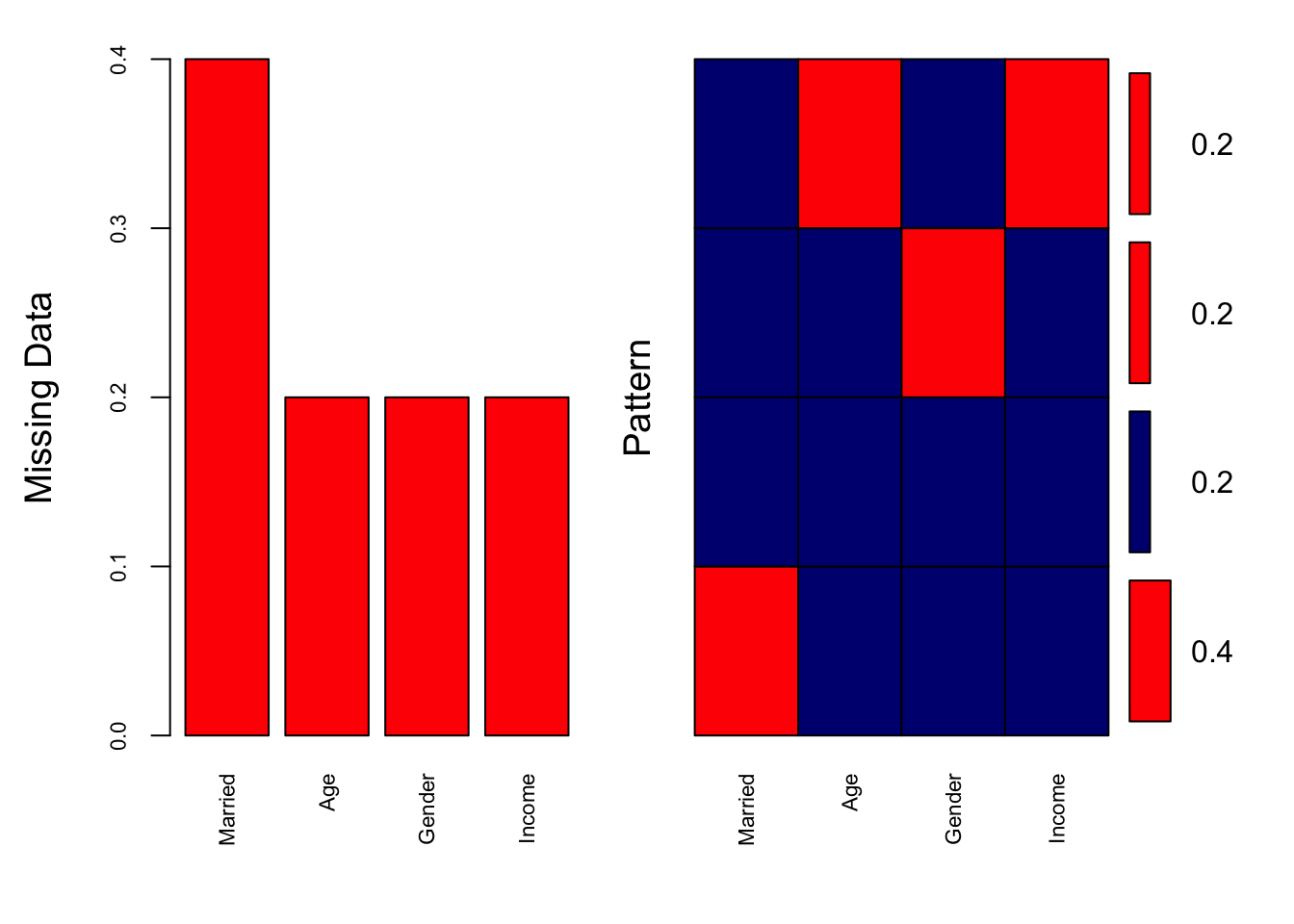


 Variables sorted by number of missings: 
 Variable Count
  Married   0.4
      Age   0.2
   Gender   0.2
   Income   0.2

#  Mean Imputation
data_mean <- data
data_mean$Age[is.na(data_mean$Age)] <- mean(data_mean$Age, na.rm = TRUE)
data_mean$Income[is.na(data_mean$Income)] <- mean(data_mean$Income, na.rm = TRUE)

#  Median Imputation
data_median <- data
data_median$Age[is.na(data_median$Age)] <- median(data_median$Age, na.rm = TRUE)
data_median$Income[is.na(data_median$Income)] <- median(data_median$Income, na.rm = TRUE)

Smaller k Imputation is influenced by fewer, closer neighbours. The imputed values may closely match the most similar existing values. Can introduce variability or bias if the nearest neighbours are not representative of the overall distribution.
Larger k Imputation is influenced by more neighbours, smoothing the imputed values. Reduces variability but may dilute local patterns, making the imputed values less specific.

#  KNN Imputation (k=3)
data_knn <- kNN(data, variable = c("Age", "Income"), k = 3)
data_knn <- data_knn[, colnames(data)]  # Remove '_imp' columns added by KNN

cat("\nAfter KNN Imputation (k=3):\n")


After KNN Imputation (k=3):

print(data_knn)

  Age Gender Income Married
1  25   Male  50000    <NA>
2  30   <NA>  60000     Yes
3  35 Female  58000      No
4  35   Male  55000     Yes
5  40 Female  58000    <NA>

#  Combine Data for ggplot2 Visualisation
# Combine original, mean, median, and KNN imputation for Age
imputed_age <- data.frame(
  Method = rep(c("Original", "Mean", "Median", "KNN"), each = nrow(data)),
  Age = c(data$Age, data_mean$Age, data_median$Age, data_knn$Age)
)

# Combine original, mean, median, and KNN imputation for Income
imputed_income <- data.frame(
  Method = rep(c("Original", "Mean", "Median", "KNN"), each = nrow(data)),
  Income = c(data$Income, data_mean$Income, data_median$Income, data_knn$Income)
)

#  Visualise Imputed Results for Age
ggplot(imputed_age, aes(x = Method, y = Age, fill = Method)) +
  geom_boxplot() +
  theme_minimal() +
  labs(title = "Comparison of Age Imputation Methods", x = "Imputation Method", y = "Age")

Warning: Removed 1 rows containing non-finite values (`stat_boxplot()`).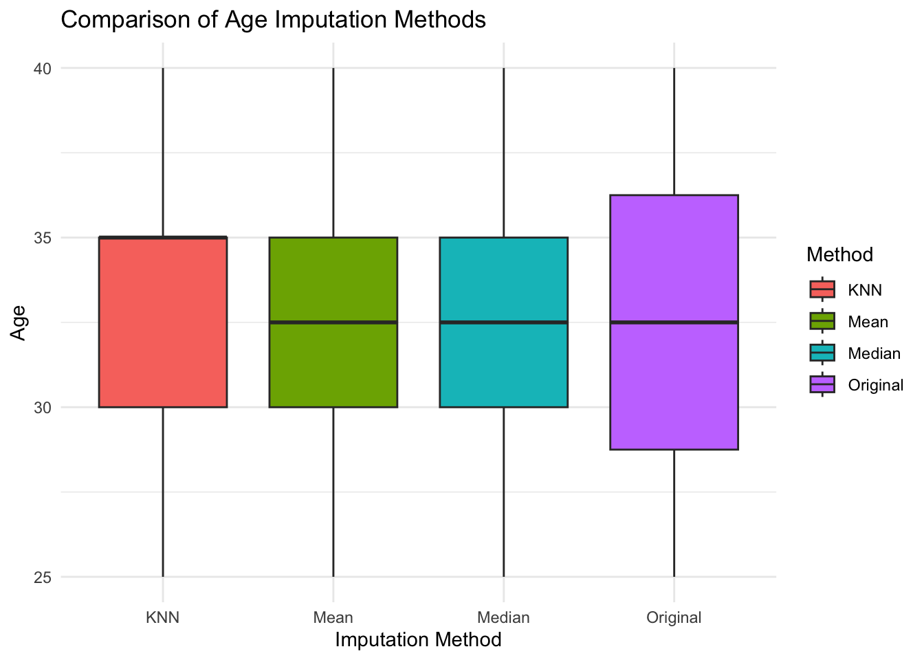

#  Visualise Imputed Results for Income
ggplot(imputed_income, aes(x = Method, y = Income, fill = Method)) +
  geom_boxplot() +
  theme_minimal() +
  labs(title = "Comparison of Income Imputation Methods", x = "Imputation Method", y = "Income") +
  scale_fill_brewer(palette = "Set3")

Warning: Removed 1 rows containing non-finite values (`stat_boxplot()`).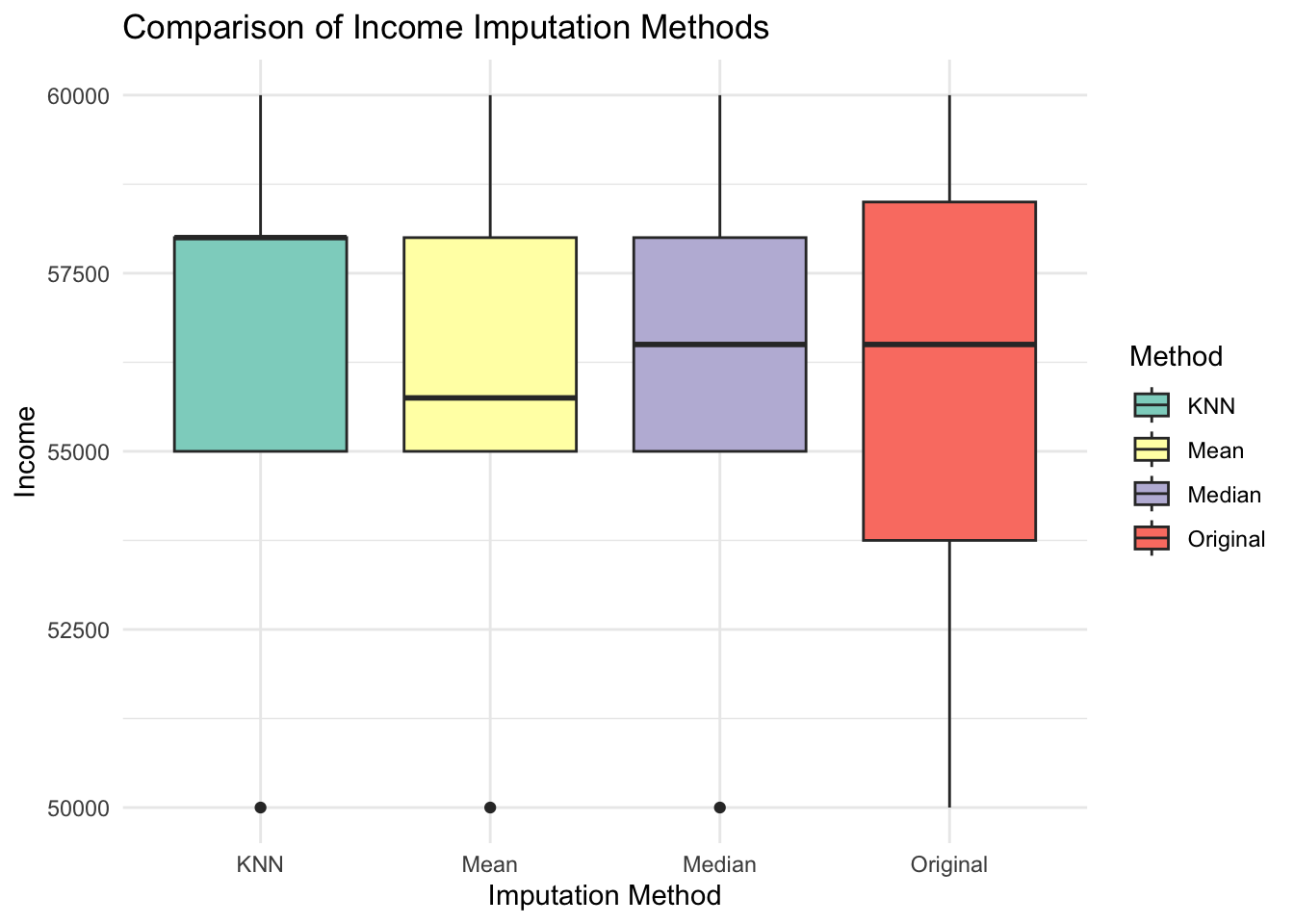

Want to understand KNN better? Check this tutorial out (PYTHON) https://www.analyticsvidhya.com/blog/2020/07/knnimputer-a-robust-way-to-impute-missing-values-using-scikit-learn/

One hot encoding

data$Gender_Male <- ifelse(data$Gender == "Male", 1, 0)
data$Gender_Female <- ifelse(data$Gender == "Female", 1, 0)

print(data)

  Age Gender Income Married Gender_Male Gender_Female
1  25   Male  50000    <NA>           1             0
2  30   <NA>  60000     Yes          NA            NA
3  NA Female     NA      No           0             1
4  35   Male  55000     Yes           1             0
5  40 Female  58000    <NA>           0             1

But what if you have more categories?

library(caret)

Loading required package: lattice

data <- data.frame(
  ID = 1:6,
  Category = c("A", "B", "C", "A", "B", "D"),
  Value = c(10, 20, 30, 40, 50, 60)
)

cat("Original Dataset:\n")

Original Dataset:

print(data)

  ID Category Value
1  1        A    10
2  2        B    20
3  3        C    30
4  4        A    40
5  5        B    50
6  6        D    60

There are other ways to do it! Other functions (e.g step_dummy() in tidymodels)

#  Create Dummy Variables (All Categories)
# Create a dummyVars object
dummy_model <- dummyVars(~ Category, data = data)

# Apply the model to the dataset
dummy_encoded <- predict(dummy_model, newdata = data)

print(dummy_encoded)

  CategoryA CategoryB CategoryC CategoryD
1         1         0         0         0
2         0         1         0         0
3         0         0         1         0
4         1         0         0         0
5         0         1         0         0
6         0         0         0         1

# Combine Encoded Variables with Original Data
# Combine dummy variables with the original dataset
data_combined <- cbind(data, dummy_encoded)
print(data_combined)

  ID Category Value CategoryA CategoryB CategoryC CategoryD
1  1        A    10         1         0         0         0
2  2        B    20         0         1         0         0
3  3        C    30         0         0         1         0
4  4        A    40         1         0         0         0
5  5        B    50         0         1         0         0
6  6        D    60         0         0         0         1

What is changing here?

#  Create Dummy Variables with Full Rank (Exclude Reference Category)
# Create a dummyVars object with fullRank = TRUE
dummy_model_reduced <- dummyVars(~ Category, data = data, fullRank = TRUE)

# Apply the model to the dataset
dummy_encoded_reduced <- predict(dummy_model_reduced, newdata = data)

print(dummy_encoded_reduced)

  CategoryB CategoryC CategoryD
1         0         0         0
2         1         0         0
3         0         1         0
4         0         0         0
5         1         0         0
6         0         0         1

# Combine reduced-rank dummy variables with the original dataset
data_combined_reduced <- cbind(data, dummy_encoded_reduced)


print(data_combined_reduced)

  ID Category Value CategoryB CategoryC CategoryD
1  1        A    10         0         0         0
2  2        B    20         1         0         0
3  3        C    30         0         1         0
4  4        A    40         0         0         0
5  5        B    50         1         0         0
6  6        D    60         0         0         1