import pandas as pd
import numpy as np
import seaborn as sns
import matplotlib.pyplot as plt
from sklearn.impute import SimpleImputer, KNNImputer
from sklearn.datasets import fetch_openml
from sklearn.compose import ColumnTransformer
from sklearn.pipeline import Pipeline
from sklearn.preprocessing import OneHotEncoder
from sklearn.preprocessing import StandardScaler, OneHotEncoder, LabelEncoder
from sklearn import set_config
set_config(display='diagram')Missing Data Imputation - Python
Missing Data Imputation
We are using both Pandas (data loading, processing, transformation and manipulation) and Scikit-learn (example data source, ML and statistical analysis)
This example illustrates how to apply different preprocessing and feature imputation pipelines to different subsets of features, using SimpleImputer and KNNImputer. This is particularly handy for the case of datasets that contain heterogeneous data types, since we may want to impute the numeric as well as categorical features.
You can download the dataset we will be using through the link:
np.random.seed(0)

## Load the LongIsland_Heart_Data Set
heart_df = pd.read_csv('/Users/bravol/Desktop/ML Class/Practical/EDA/LongIsland_Heart_Data.csv') #change to your own directory

heart_df.describe() #similar to summary()
age sex ... thal diagnosis of heart disease
count 180.000000 180.000000 ... 180.000000 200.000000
mean 59.472222 0.966667 ... 1.411111 2.520000
std 7.718823 0.180006 ... 0.967568 1.219441
min 35.000000 0.000000 ... 1.000000 1.000000
25% 55.000000 1.000000 ... 1.000000 1.000000
50% 60.000000 1.000000 ... 1.000000 2.000000
75% 64.000000 1.000000 ... 1.000000 4.000000
max 77.000000 1.000000 ... 4.000000 5.000000
[8 rows x 14 columns]print(heart_df) age sex cp trestbps ... slope ca thal diagnosis of heart disease
0 63.0 1.0 4.0 10.0 ... 3.0 1.0 1.0 3
1 44.0 1.0 4.0 3.0 ... 1.0 NaN 1.0 1
2 60.0 1.0 4.0 5.0 ... 4.0 1.0 NaN 3
3 55.0 1.0 4.0 11.0 ... 2.0 1.0 1.0 2
4 66.0 1.0 3.0 33.0 ... 3.0 1.0 1.0 1
.. ... ... ... ... ... ... ... ... ...
195 54.0 0.0 4.0 41.0 ... 1.0 1.0 1.0 2
196 62.0 1.0 1.0 1.0 ... 1.0 1.0 1.0 1
197 55.0 1.0 4.0 37.0 ... 1.0 NaN 3.0 3
198 58.0 1.0 NaN 1.0 ... 1.0 1.0 1.0 1
199 62.0 1.0 2.0 34.0 ... 1.0 1.0 NaN 2
[200 rows x 14 columns]Now let’s make a smaller dataset with just 4 features:
Numeric Features:
-
chol: numeric; – serum cholestoral in mg/dl -
thalach: numeric – maximum heart rate achieved
Categorical Features:
-
sex: categories encoded as numeric{'1 = male', '2=female'}; -
cp: ordinal integers{1, 2, 3, 4}. – Value 1: typical angina – Value 2: atypical angina – Value 3: non-anginal pain – Value 4: asymptomatic
X_reduced = heart_df.loc[:, ['chol', 'thalach','sex','cp']]
print(X_reduced)
chol thalach sex cp
0 60.0 12.0 1.0 4.0
1 NaN 8.0 1.0 4.0
2 27.0 19.0 1.0 4.0
3 39.0 25.0 1.0 4.0
4 22.0 53.0 1.0 3.0
.. ... ... ... ...
195 95.0 NaN 0.0 4.0
196 30.0 1.0 1.0 1.0
197 33.0 4.0 1.0 4.0
198 3.0 1.0 1.0 NaN
199 NaN 47.0 1.0 2.0
[200 rows x 4 columns]Visualize Missingness
sns.heatmap(X_reduced.isnull(), cbar=False, cmap="viridis")
plt.title("Missing Values Heatmap")
plt.show()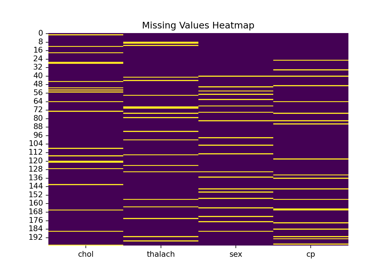
Impute Missing Values with SimpleImputer
For more information on imputation in python go to https://scikit-learn.org/1.5/modules/generated/sklearn.impute.SimpleImputer.html
# Define numeric and categorical features
numeric_features = ['chol', 'thalach']
categorical_features = ['sex','cp']
Make sure categorical values are interpreted as categorical
X_reduced.dtypeschol float64
thalach float64
sex float64
cp float64
dtype: objectX_reduced[categorical_features] = X_reduced[categorical_features].astype('category')X_reduced.dtypeschol float64
thalach float64
sex category
cp category
dtype: object# Impute numeric features with the mean
numeric_imputer = SimpleImputer(strategy='median')
X_reduced[numeric_features] = numeric_imputer.fit_transform(X_reduced[numeric_features])
print(X_reduced) chol thalach sex cp
0 60.0 12.0 1.0 4.0
1 29.0 8.0 1.0 4.0
2 27.0 19.0 1.0 4.0
3 39.0 25.0 1.0 4.0
4 22.0 53.0 1.0 3.0
.. ... ... ... ...
195 95.0 19.0 0.0 4.0
196 30.0 1.0 1.0 1.0
197 33.0 4.0 1.0 4.0
198 3.0 1.0 1.0 NaN
199 29.0 47.0 1.0 2.0
[200 rows x 4 columns]# Impute categorical features with a constant value ('Unknown')
categorical_imputer = SimpleImputer(strategy='constant', fill_value=-1)
X_reduced[categorical_features] = categorical_imputer.fit_transform(X_reduced[categorical_features])
print(X_reduced) chol thalach sex cp
0 60.0 12.0 1.0 4.0
1 29.0 8.0 1.0 4.0
2 27.0 19.0 1.0 4.0
3 39.0 25.0 1.0 4.0
4 22.0 53.0 1.0 3.0
.. ... ... ... ...
195 95.0 19.0 0.0 4.0
196 30.0 1.0 1.0 1.0
197 33.0 4.0 1.0 4.0
198 3.0 1.0 1.0 -1.0
199 29.0 47.0 1.0 2.0
[200 rows x 4 columns]Visualize the imputation. Has it worked?
sns.heatmap(X_reduced.isnull(), cbar=False, cmap="viridis")
plt.title("Missing Values Heatmap")
plt.show()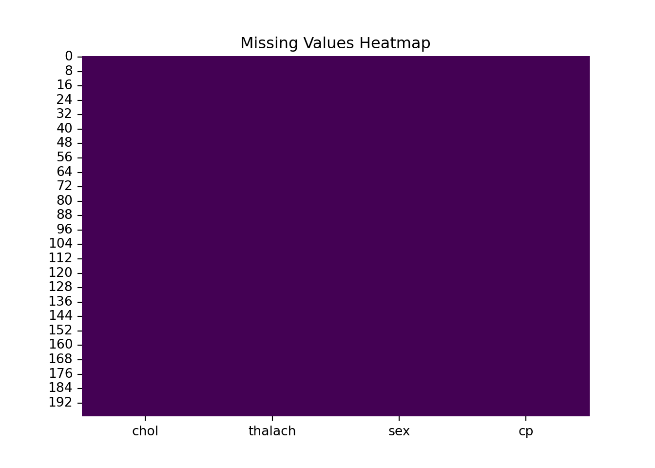
Now impute Missing Values with KNNImputer (for Numeric Data)
X_reduced_KNN = heart_df.loc[:, ['chol', 'thalach','sex','cp']]

knn_imputer = KNNImputer(n_neighbors=5)
X_reduced_KNN[numeric_features] = knn_imputer.fit_transform(X_reduced_KNN[numeric_features])
What difference can we see in the datasets? Compare Summary Statistics Before and After Imputation
X_reduced_KNN.describe() chol thalach sex cp
count 200.000000 200.000000 180.000000 180.000000
mean 36.811000 23.669000 0.966667 3.500000
std 28.606273 20.140448 0.180006 0.794534
min 1.000000 1.000000 0.000000 1.000000
25% 6.000000 3.750000 1.000000 3.000000
50% 31.500000 19.000000 1.000000 4.000000
75% 58.250000 41.250000 1.000000 4.000000
max 100.000000 60.000000 1.000000 4.000000X_reduced.describe() chol thalach sex cp
count 200.000000 200.00000 200.000000 200.000000
mean 35.655000 23.20000 0.770000 3.050000
std 28.449655 20.09275 0.615626 1.549031
min 1.000000 1.00000 -1.000000 -1.000000
25% 6.000000 3.75000 1.000000 3.000000
50% 29.000000 19.00000 1.000000 4.000000
75% 57.250000 41.25000 1.000000 4.000000
max 100.000000 60.00000 1.000000 4.000000Dummy variables
As well as imputation we are interested in other transformations. For example, hot encoding categorical data. For extra insight https://www.kaggle.com/code/marcinrutecki/one-hot-encoding-everything-you-need-to-know
X_reduced_Encoder = heart_df.loc[:, ['chol', 'thalach','sex','cp']]
X_reduced_Encoder[categorical_features] = X_reduced_Encoder[categorical_features].astype('category')

# Apply OneHotEncoder
encoder = OneHotEncoder(handle_unknown='ignore', sparse_output=False)
encoded_categorical = encoder.fit_transform(X_reduced_Encoder[categorical_features])
encoded_df = pd.DataFrame(
encoded_categorical,
columns=encoder.get_feature_names_out(categorical_features)
)# Combine the encoded features with the original dataset (drop original categorical columns)
visualised_df = pd.concat([X_reduced_Encoder.drop(columns=categorical_features), encoded_df], axis=1)
print(visualised_df) chol thalach sex_0.0 sex_1.0 ... cp_2.0 cp_3.0 cp_4.0 cp_nan
0 60.0 12.0 0.0 1.0 ... 0.0 0.0 1.0 0.0
1 NaN 8.0 0.0 1.0 ... 0.0 0.0 1.0 0.0
2 27.0 19.0 0.0 1.0 ... 0.0 0.0 1.0 0.0
3 39.0 25.0 0.0 1.0 ... 0.0 0.0 1.0 0.0
4 22.0 53.0 0.0 1.0 ... 0.0 1.0 0.0 0.0
.. ... ... ... ... ... ... ... ... ...
195 95.0 NaN 1.0 0.0 ... 0.0 0.0 1.0 0.0
196 30.0 1.0 0.0 1.0 ... 0.0 0.0 0.0 0.0
197 33.0 4.0 0.0 1.0 ... 0.0 0.0 1.0 0.0
198 3.0 1.0 0.0 1.0 ... 0.0 0.0 0.0 1.0
199 NaN 47.0 0.0 1.0 ... 1.0 0.0 0.0 0.0
[200 rows x 10 columns]As you have seen we have gone back to original data so one of the new columns created is nan! To circumvent this apply this to a dataframe AFTER imputation!!!
#Impute dataset and then do the hot encoding: Check out the concept of Pipeline https://scikit-learn.org/1.5/modules/generated/sklearn.pipeline.Pipeline.html when do you think it can come in handy?