HDS MSc - Module 3 - PreProcessing/EDA

Data wrangling with R

This code is based on the original work from HealthyR and has been adapted by Laura Bravo

Tidyverse packages: ggplot2, dplyr, tidyr, etc.

Most of the functions introduced in this session come from the tidyverse family, rather than Base R. Including library(tidyverse) in your script loads a list of packages: ggplot2, dplyr, tidyr, forcats, etc.

library(tidyverse)

── Attaching core tidyverse packages ──────────────────────── tidyverse 2.0.0 ──
✔ dplyr     1.1.2     ✔ readr     2.1.4
✔ forcats   1.0.0     ✔ stringr   1.5.0
✔ ggplot2   3.4.3     ✔ tibble    3.2.1
✔ lubridate 1.9.2     ✔ tidyr     1.3.0
✔ purrr     1.0.1     
── Conflicts ────────────────────────────────────────── tidyverse_conflicts() ──
✖ dplyr::filter() masks stats::filter()
✖ dplyr::lag()    masks stats::lag()
ℹ Use the conflicted package (<http://conflicted.r-lib.org/>) to force all conflicts to become errors

In this session we will get to know key functions to work with data:

summarise data using: group_by(), summarise(), and mutate();
reshape data between the wide and long formats: pivot_wider() and pivot_longer();
select() columns and arrange() (sort) rows.

Data

We are using a condensed version of the Global Burden of Disease Data dataset.

#Can load the dataset through many ways but quickest and one i always resort to, is data.table function
library(data.table)


Attaching package: 'data.table'

The following objects are masked from 'package:lubridate':

    hour, isoweek, mday, minute, month, quarter, second, wday, week,
    yday, year

The following objects are masked from 'package:dplyr':

    between, first, last

The following object is masked from 'package:purrr':

    transpose

gbd_full <- fread("global_burden_disease_cause-year-sex-income.csv") #add your working directory

head(gbd_full)

                   cause year    sex       income deaths_millions
1: Communicable diseases 1990 Female         High            0.21
2: Communicable diseases 1990 Female Upper-Middle            1.15
3: Communicable diseases 1990 Female Lower-Middle            4.43
4: Communicable diseases 1990 Female          Low            1.51
5: Communicable diseases 1990   Male         High            0.26
6: Communicable diseases 1990   Male Upper-Middle            1.35

# Creating a single-year tibble for printing and simple examples:
gbd2017 <- gbd_full %>% 
  filter(year == "2017")

Plot the data

The best way to investigate a dataset is to plot it (do not worry if do not understand the code, will do a separate exercise on plotting later)

gbd2017 %>% 
  # without the mutate(... = fct_relevel()) 
  # the panels get ordered alphabetically
  mutate(income = fct_relevel(income,
                              "Low",
                              "Lower-Middle",
                              "Upper-Middle",
                              "High")) %>% 
  # defining the variables using ggplot(aes(...)):
  ggplot(aes(x = sex, y = deaths_millions, fill = cause)) +
  # type of geom to be used: column (that's a type of barplot):
  geom_col(position = "dodge") +
  # facets for the income groups:
  facet_wrap(~income, ncol = 4) +
  # move the legend to the top of the plot (default is "right"):
  theme(legend.position = "top")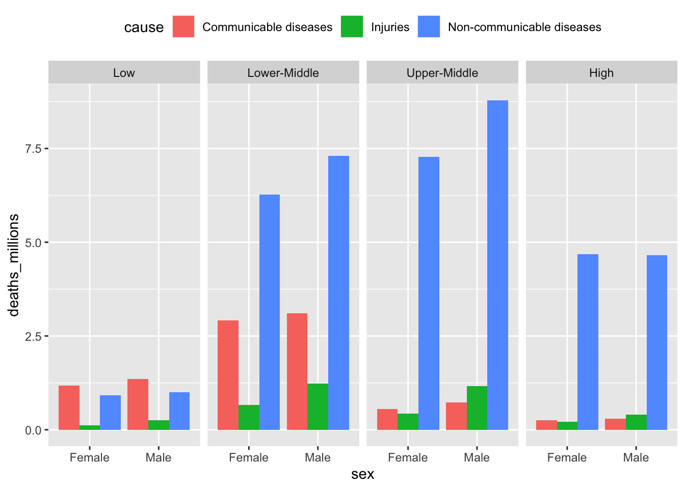

Aggregating: `group_by()`, `summarise()`

Health data analysis is frequently concerned with making comparisons between groups. Groups of genes, or diseases, or patients, or populations, etc. An easy approach to the comparison of data by a categorical grouping is therefore essential.

We will introduce flexible functions from tidyverse that you can apply in any setting.

To quickly calculate the total number of deaths in 2017, we can select the column and send it into the sum() function:

gbd2017$deaths_millions %>% sum()

[1] 55.74

But a much cleverer way of summarising data is using the summarise() function:

gbd2017 %>% 
  summarise(sum(deaths_millions))

  sum(deaths_millions)
1                55.74

sum() is a function that adds numbers together, whereas summarise() is an efficient way of creating summarised dataframes. The main strength of summarise() is how it works with the group_by() function. group_by() and summarise() are a perfect complement for each other and used togetehr most of the time.

We use group_by() to tell summarise() which subgroups to apply the calculations on. In the above example, without group_by(), summarise just works on the whole dataset, yielding the same result as just sending a single column into the sum() function.

We can subset on the cause variable using group_by():

gbd2017 %>% 
  group_by(cause) %>% 
  summarise(sum(deaths_millions))

# A tibble: 3 × 2
  cause                     `sum(deaths_millions)`
  <chr>                                      <dbl>
1 Communicable diseases                      10.4 
2 Injuries                                    4.47
3 Non-communicable diseases                  40.9

Furthermore, group_by() is happy to accept multiple grouping variables. So by just copying and editing the above code, we can quickly get summarised totals across multiple grouping variables (by just adding sex inside the group_by() after cause):

gbd2017 %>% 
  group_by(cause, sex) %>% 
  summarise(sum(deaths_millions))

`summarise()` has grouped output by 'cause'. You can override using the
`.groups` argument.

# A tibble: 6 × 3
# Groups:   cause [3]
  cause                     sex    `sum(deaths_millions)`
  <chr>                     <chr>                   <dbl>
1 Communicable diseases     Female                   4.91
2 Communicable diseases     Male                     5.47
3 Injuries                  Female                   1.42
4 Injuries                  Male                     3.05
5 Non-communicable diseases Female                  19.2 
6 Non-communicable diseases Male                    21.7

Add new columns: `mutate()`

Let’s first give the summarised column a better name, e.g., deaths_per_group. We can remove groupings by using ungroup(). This is important to remember if you want to manipulate the dataset in its original format. We can combine ungroup() with mutate() to add a total deaths column, which will be used below to calculate a percentage:

gbd2017 %>% 
  group_by(cause, sex) %>% 
  summarise(deaths_per_group = sum(deaths_millions)) %>% 
  ungroup() %>% 
  mutate(deaths_total = sum(deaths_per_group))

`summarise()` has grouped output by 'cause'. You can override using the
`.groups` argument.

# A tibble: 6 × 4
  cause                     sex    deaths_per_group deaths_total
  <chr>                     <chr>             <dbl>        <dbl>
1 Communicable diseases     Female             4.91         55.7
2 Communicable diseases     Male               5.47         55.7
3 Injuries                  Female             1.42         55.7
4 Injuries                  Male               3.05         55.7
5 Non-communicable diseases Female            19.2          55.7
6 Non-communicable diseases Male              21.7          55.7

So summarise() condenses a dataframe, whereas mutate() retains its current size and adds columns.

Percentages formatting: `percent()`

We can also add further lines to mutate() to calculate the percentage of each group:

# percent() function for formatting percentages come from library(scales)
library(scales)
gbd2017_summarised <- gbd2017 %>% 
  group_by(cause, sex) %>% 
  summarise(deaths_per_group = sum(deaths_millions)) %>% 
  ungroup() %>% 
  mutate(deaths_total    = sum(deaths_per_group),
        deaths_relative = deaths_per_group/deaths_total)
gbd2017_summarised

# A tibble: 6 × 5
  cause                     sex    deaths_per_group deaths_total deaths_relative
  <chr>                     <chr>             <dbl>        <dbl>           <dbl>
1 Communicable diseases     Female             4.91         55.7          0.0881
2 Communicable diseases     Male               5.47         55.7          0.0981
3 Injuries                  Female             1.42         55.7          0.0255
4 Injuries                  Male               3.05         55.7          0.0547
5 Non-communicable diseases Female            19.2          55.7          0.344 
6 Non-communicable diseases Male              21.7          55.7          0.390

`summarise()` vs `mutate()`

So far we’ve shown you examples of using summarise() on grouped data (following group_by()) and mutate() on the whole dataset (without using group_by()).

But here’s the thing: mutate() is also happy to work on grouped data.

Let’s save the aggregated example from above in a new dataframe. We will then sort the rows using arrange() based on sex, just for easier viewing (it was previously sorted by cause).

The arrange() function sorts the rows within a tibble:

gbd_summarised <- gbd2017 %>% 
  group_by(cause, sex) %>% 
  summarise(deaths_per_group = sum(deaths_millions)) %>% 
  arrange(sex)

`summarise()` has grouped output by 'cause'. You can override using the
`.groups` argument.

gbd_summarised

# A tibble: 6 × 3
# Groups:   cause [3]
  cause                     sex    deaths_per_group
  <chr>                     <chr>             <dbl>
1 Communicable diseases     Female             4.91
2 Injuries                  Female             1.42
3 Non-communicable diseases Female            19.2 
4 Communicable diseases     Male               5.47
5 Injuries                  Male               3.05
6 Non-communicable diseases Male              21.7

You should also notice that summarise() drops all variables that are not listed in group_by() or created inside it. So year, income, and deaths_millions exist in gbd2017, but they do not exist in gbd_summarised.

We now want to calculate the percentage of deaths from each cause for each gender. We could use summarise() to calculate the totals:

gbd_summarised_sex <- gbd_summarised %>% 
  group_by(sex) %>% 
  summarise(deaths_per_sex = sum(deaths_per_group))

gbd_summarised_sex

# A tibble: 2 × 2
  sex    deaths_per_sex
  <chr>           <dbl>
1 Female           25.5
2 Male             30.3

But that drops the cause and deaths_per_group columns. One way would be to now use a join on gbd_summarised and gbd_summarised_sex:

full_join(gbd_summarised, gbd_summarised_sex)

Joining with `by = join_by(sex)`

# A tibble: 6 × 4
# Groups:   cause [3]
  cause                     sex    deaths_per_group deaths_per_sex
  <chr>                     <chr>             <dbl>          <dbl>
1 Communicable diseases     Female             4.91           25.5
2 Injuries                  Female             1.42           25.5
3 Non-communicable diseases Female            19.2            25.5
4 Communicable diseases     Male               5.47           30.3
5 Injuries                  Male               3.05           30.3
6 Non-communicable diseases Male              21.7            30.3

Joining different summaries together can be useful, especially if the individual pipelines are quite long (e.g., over 5 lines of %>%). However, it does increase the chance of mistakes creeping in and is best avoided if possible.

An alternative is to use mutate() with group_by() to achieve the same result as the full_join() above:

gbd_summarised %>% 
  group_by(sex) %>% 
  mutate(deaths_per_sex = sum(deaths_per_group))

# A tibble: 6 × 4
# Groups:   sex [2]
  cause                     sex    deaths_per_group deaths_per_sex
  <chr>                     <chr>             <dbl>          <dbl>
1 Communicable diseases     Female             4.91           25.5
2 Injuries                  Female             1.42           25.5
3 Non-communicable diseases Female            19.2            25.5
4 Communicable diseases     Male               5.47           30.3
5 Injuries                  Male               3.05           30.3
6 Non-communicable diseases Male              21.7            30.3

So mutate() calculates the sums within each grouping variable (in this example just group_by(sex)) and puts the results in a new column without condensing the tibble down or removing any of the existing columns.

Let’s combine all of this together into a single pipeline and calculate the percentages per cause for each gender:

gbd2017 %>% 
  group_by(cause, sex) %>% 
  summarise(deaths_per_group = sum(deaths_millions)) %>% 
  group_by(sex) %>% 
  mutate(deaths_per_sex  = sum(deaths_per_group),
         sex_cause_perc = percent(deaths_per_group/deaths_per_sex)) %>% 
  arrange(sex, deaths_per_group)

`summarise()` has grouped output by 'cause'. You can override using the
`.groups` argument.

# A tibble: 6 × 5
# Groups:   sex [2]
  cause                     sex   deaths_per_group deaths_per_sex sex_cause_perc
  <chr>                     <chr>            <dbl>          <dbl> <chr>         
1 Injuries                  Fema…             1.42           25.5 6%            
2 Communicable diseases     Fema…             4.91           25.5 19%           
3 Non-communicable diseases Fema…            19.2            25.5 75%           
4 Injuries                  Male              3.05           30.3 10.1%         
5 Communicable diseases     Male              5.47           30.3 18.1%         
6 Non-communicable diseases Male             21.7            30.3 71.8%

Common arithmetic functions - `sum()`, `mean()`, `median()`, etc.

Statistics is an R strength, so if there is an arithmetic function you can think of, it probably exists in R.

The most common ones are:

sum()
mean()
median()
min(), max()
sd() - standard deviation
IQR() - interquartile range

An import thing to remember relates to missing data: if any of your values is NA (not available; missing), these functions will return an NA. Either deal with your missing values beforehand (recommended) or add the na.rm = TRUE argument into any of the functions to ask R to ignore missing values.

mynumbers <- c(1, 2, NA)
sum(mynumbers)

[1] NA

sum(mynumbers, na.rm = TRUE)

[1] 3

`select()` columns

The select() function can be used to choose, rename, or reorder columns of a tibble.

For the following select() examples, let’s create a new tibble called gbd_2rows by taking the first 2 rows of gbd_full (just for shorter printing):

gbd_2rows <- gbd_full %>% 
  slice(1:2)

gbd_2rows

                   cause year    sex       income deaths_millions
1: Communicable diseases 1990 Female         High            0.21
2: Communicable diseases 1990 Female Upper-Middle            1.15

Let’s select() two of these columns:

gbd_2rows %>% 
  select(cause, deaths_millions)

                   cause deaths_millions
1: Communicable diseases            0.21
2: Communicable diseases            1.15

We can also use select() to rename the columns we are choosing:

gbd_2rows %>% 
  select(cause, deaths = deaths_millions)

                   cause deaths
1: Communicable diseases   0.21
2: Communicable diseases   1.15

The function rename() is similar to select(), but it keeps all variables whereas select() only kept the ones we mentioned:

gbd_2rows %>% 
  rename(deaths = deaths_millions)

                   cause year    sex       income deaths
1: Communicable diseases 1990 Female         High   0.21
2: Communicable diseases 1990 Female Upper-Middle   1.15

select() can also be used to reorder the columns in your tibble. Moving columns around is not relevant in data analysis (as any of the functions we showed you above, as well as plotting, only look at the column names, and not their positions in the tibble), but it is useful for organising your tibble for easier viewing.

So if we use select like this:

gbd_2rows %>% 
  select(year, sex, income, cause, deaths_millions)

   year    sex       income                 cause deaths_millions
1: 1990 Female         High Communicable diseases            0.21
2: 1990 Female Upper-Middle Communicable diseases            1.15

The columns are reordered.

If you want to move specific column(s) to the front of the tibble, do:

gbd_2rows %>% 
  select(year, sex, everything())

   year    sex                 cause       income deaths_millions
1: 1990 Female Communicable diseases         High            0.21
2: 1990 Female Communicable diseases Upper-Middle            1.15

And this is where the true power of select() starts to come out. In addition to listing the columns explicitly (e.g., mydata %>% select(year, cause...)) there are several special functions that can be used inside select(). These special functions are called select helpers, and the first select helper we used is everything().

The most common select helpers are starts_with(), ends_with(), contains(), matches() (but there are several others that may be useful to you, so press F1 on select() for a full list, or search the web for more examples).

Let’s say you can’t remember whether the deaths column was called deaths_millions or just deaths or deaths_mil, or maybe there are other columns that include the word “deaths” that you want to select():

gbd_2rows %>% 
  select(starts_with("deaths"))

   deaths_millions
1:            0.21
2:            1.15

Note how “deaths” needs to be quoted inside starts_with() - as it’s a word to look for, not the real name of a column/variable.

Reshaping data - long vs wide format

So far, all of the examples we’ve shown you have been using ‘tidy’ data. Data is ‘tidy’ when it follows a couple of rules: each variable is in its own column, and each observation is in its own row. Making data ‘tidy’ often means transforming the table from a “wide” format into a “long” format. Long format is efficient to use in data analysis and visualisation and can also be considered “computer readable”.

But sometimes when presenting data in tables for humans to read, or when collecting data directly into a spreadsheet, it can be convenient to have data in a wide format. Data is ‘wide’ when some or all of the columns are levels of a factor. An example makes this easier to see.

gbd_wide <- read_csv("global_burden_disease_wide-format.csv") #add your wd
gbd_long <- read_csv("global_burden_disease_cause-year-sex.csv")  ##add your wd

head(gbd_wide)

# A tibble: 3 × 5
  cause                     Female_1990 Female_2017 Male_1990 Male_2017
  <chr>                           <dbl>       <dbl>     <dbl>     <dbl>
1 Communicable diseases            7.3         4.91      8.06      5.47
2 Injuries                         1.41        1.42      2.84      3.05
3 Non-communicable diseases       12.8        19.2      13.9      21.7

head(gbd_long)

# A tibble: 6 × 4
  cause                  year sex    deaths_millions
  <chr>                 <dbl> <chr>            <dbl>
1 Communicable diseases  1990 Female            7.3 
2 Communicable diseases  2017 Female            4.91
3 Communicable diseases  1990 Male              8.06
4 Communicable diseases  2017 Male              5.47
5 Injuries               1990 Female            1.41
6 Injuries               2017 Female            1.42

These tables contain the exact same information, but in long (tidy) and wide formats, respectively.

Pivot values from rows into columns (wider)

If we want to take the long data and put some of the numbers next to each other for easier visualisation, then pivot_wider() from the tidyr package is the function to do it. It means we want to send a variable into columns, and it needs just two arguments: the variable we want to become the new columns, and the variable where the values currently are.

gbd_long %>% 
  pivot_wider(names_from = year, values_from = deaths_millions)

# A tibble: 6 × 4
  cause                     sex    `1990` `2017`
  <chr>                     <chr>   <dbl>  <dbl>
1 Communicable diseases     Female   7.3    4.91
2 Communicable diseases     Male     8.06   5.47
3 Injuries                  Female   1.41   1.42
4 Injuries                  Male     2.84   3.05
5 Non-communicable diseases Female  12.8   19.2 
6 Non-communicable diseases Male    13.9   21.7

This means we can quickly eyeball how the number of deaths has changed from 1990 to 2017 for each cause category and sex. Whereas if we wanted to quickly look at the difference in the number of deaths for females and males, we can change the names_from = argument from = years to = sex. Furthermore, we can also add a mutate() to calculate the difference:

gbd_long %>% 
  pivot_wider(names_from = sex, values_from = deaths_millions) %>% 
  mutate(Male - Female)

# A tibble: 6 × 5
  cause                      year Female  Male `Male - Female`
  <chr>                     <dbl>  <dbl> <dbl>           <dbl>
1 Communicable diseases      1990   7.3   8.06           0.760
2 Communicable diseases      2017   4.91  5.47           0.560
3 Injuries                   1990   1.41  2.84           1.43 
4 Injuries                   2017   1.42  3.05           1.63 
5 Non-communicable diseases  1990  12.8  13.9            1.11 
6 Non-communicable diseases  2017  19.2  21.7            2.59

All of these differences are positive which means every year, more men die than women. Which make sense, as more boys are born than girls.

And what if we want to look at both year and sex at the same time? No problem, pivot_wider() can deal with multiple variables at the same time, names_from = c(sex, year):

gbd_long %>% 
  pivot_wider(names_from = c(sex, year), values_from = deaths_millions)

# A tibble: 3 × 5
  cause                     Female_1990 Female_2017 Male_1990 Male_2017
  <chr>                           <dbl>       <dbl>     <dbl>     <dbl>
1 Communicable diseases            7.3         4.91      8.06      5.47
2 Injuries                         1.41        1.42      2.84      3.05
3 Non-communicable diseases       12.8        19.2      13.9      21.7

pivot_wider() has a few optional arguments that may be useful for you. For example, pivot_wider(..., values_fill = 0) can be used to fill empty cases (if you have any) with a value you specified. Or pivot_wider(..., names_sep = ": ") can be used to change the separator that gets put between the values (e.g., you may want “Female: 1990” instead of the default “Female_1990”). Remember that pressing F1 when your cursor is on a function opens it up in the Help tab where these extra options are listed.

Pivot values from columns to rows (longer)

The inverse of pivot_wider() is pivot_longer(). If you’re lucky enough, your data comes from a proper database and is already in the long and tidy format. But if not you’ll need to know how to wrangle the variables currently spread across different columns into the tidy format (where each column is a variable, each row is an observation).

pivot_longer() can be a little bit more difficult to use as you need to describe all the columns to be collected using a select_helper. Run `?select_helpers and click on the first result in the Help tab for a reminder.

For example, here we want to collect all the columns that include the words Female or Male, the select helper for it is matches("Female|Male"):

gbd_wide %>% 
  pivot_longer(matches("Female|Male"), 
               names_to = "sex_year", 
               values_to = "deaths_millions") %>% 
  slice(1:6)

# A tibble: 6 × 3
  cause                 sex_year    deaths_millions
  <chr>                 <chr>                 <dbl>
1 Communicable diseases Female_1990            7.3 
2 Communicable diseases Female_2017            4.91
3 Communicable diseases Male_1990              8.06
4 Communicable diseases Male_2017              5.47
5 Injuries              Female_1990            1.41
6 Injuries              Female_2017            1.42

You’re probably looking at the example above and thinking that’s all nice and simple on this miniature example dataset, but how on earth will I figure this out on a real-world example. And you’re right, we won’t deny that pivot_longer() is one of the most technically complicated functions in this book, and it can take a lot of trial and error to get it to work. How to get started with your own pivot_longer() transformation is to first play with the select() function to make sure you are telling R exactly which columns to pivot into the longer format. For example, before working out the pivot_longer() code for the above example, we would figure this out first:

gbd_wide %>% 
  select(matches("Female|Male"))

# A tibble: 3 × 4
  Female_1990 Female_2017 Male_1990 Male_2017
        <dbl>       <dbl>     <dbl>     <dbl>
1        7.3         4.91      8.06      5.47
2        1.41        1.42      2.84      3.05
3       12.8        19.2      13.9      21.7

Then, knowing that matches("Female|Male") works as expected inside our little select() test, we can copy-paste it into pivot_longer() and add the names_to and values_to arguments. Both of these arguments are new column names that you can make up (in the above example, we are using “sex_year” and “deaths_millions”).

`separate()` a column into multiple columns

While pivot_longer() did a great job fetching the different observations that were spread across multiple columns into a single one, it’s still a combination of two variables - sex and year. We can use the separate() function to deal with that.

gbd_wide %>% 
  # same pivot_longer as before
  pivot_longer(matches("Female|Male"), 
               names_to = "sex_year", 
               values_to = "deaths_millions") %>% 
  separate(sex_year, into = c("sex", "year"), sep = "_", convert = TRUE)

# A tibble: 12 × 4
   cause                     sex     year deaths_millions
   <chr>                     <chr>  <int>           <dbl>
 1 Communicable diseases     Female  1990            7.3 
 2 Communicable diseases     Female  2017            4.91
 3 Communicable diseases     Male    1990            8.06
 4 Communicable diseases     Male    2017            5.47
 5 Injuries                  Female  1990            1.41
 6 Injuries                  Female  2017            1.42
 7 Injuries                  Male    1990            2.84
 8 Injuries                  Male    2017            3.05
 9 Non-communicable diseases Female  1990           12.8 
10 Non-communicable diseases Female  2017           19.2 
11 Non-communicable diseases Male    1990           13.9 
12 Non-communicable diseases Male    2017           21.7

We’ve also added convert = TRUE to separate() so year would get converted into a numeric variable. The combination of, e.g., “Female-1990” is a character variable, so after separating them both sex and year would still be classified as characters. But the convert = TRUE recognises that year is a number and will appropriately convert it into an integer.

`arrange()` rows

The arrange() function sorts rows based on the column(s) you want. By default, it arranges the tibble in ascending order:

gbd_long %>% 
  arrange(deaths_millions) %>% 
  # first 3 rows just for printing:
  slice(1:3)

# A tibble: 3 × 4
  cause     year sex    deaths_millions
  <chr>    <dbl> <chr>            <dbl>
1 Injuries  1990 Female            1.41
2 Injuries  2017 Female            1.42
3 Injuries  1990 Male              2.84

For numeric variables, we can just use a - to sort in descending order:

gbd_long %>% 
  arrange(-deaths_millions) %>% 
  slice(1:3)

# A tibble: 3 × 4
  cause                      year sex    deaths_millions
  <chr>                     <dbl> <chr>            <dbl>
1 Non-communicable diseases  2017 Male              21.7
2 Non-communicable diseases  2017 Female            19.2
3 Non-communicable diseases  1990 Male              13.9

The - doesn’t work for categorical variables; they need to be put in desc() for arranging in descending order:

gbd_long %>% 
  arrange(desc(sex)) %>% 
  # printing rows 1, 2, 11, and 12
  slice(1,2, 11, 12)

# A tibble: 4 × 4
  cause                      year sex    deaths_millions
  <chr>                     <dbl> <chr>            <dbl>
1 Communicable diseases      1990 Male              8.06
2 Communicable diseases      2017 Male              5.47
3 Non-communicable diseases  1990 Female           12.8 
4 Non-communicable diseases  2017 Female           19.2

Factor levels

arrange() sorts characters alphabetically, whereas factors will be sorted by the order of their levels. Let’s make the cause column into a factor:

gbd_factored <- gbd_long %>% 
  mutate(cause = factor(cause))

When we first create a factor, its levels will be ordered alphabetically:

gbd_factored$cause %>% levels()

[1] "Communicable diseases"     "Injuries"                 
[3] "Non-communicable diseases"

But we can now use fct_relevel() inside mutate() to change the order of these levels:

gbd_factored <- gbd_factored %>% 
  mutate(cause = cause %>% 
           fct_relevel("Injuries"))

gbd_factored$cause %>% levels()

[1] "Injuries"                  "Communicable diseases"    
[3] "Non-communicable diseases"

fct_relevel() brings the level(s) listed in it to the front.

So if we use arrange() on gbd_factored, the cause column will be sorted based on the order of its levels, not alphabetically. This is especially useful in two places:

plotting - categorical variables that are characters will be ordered alphabetically (e.g., think barplots), regardless of whether the rows are arranged or not;
statistical tests - the reference level of categorical variables that are characters is the alphabetically first (e.g., what the odds ratio is relative to).

However, making a character column into a factor gives us power to give its levels a non-alphabetical order, giving us control over plotting order or defining our reference levels for use in statistical tests.

Exercises

Exercise - `pivot_wider()`

Using the GBD dataset with variables cause, year (1990 and 2017 only), sex :

gbd_long <- read_csv("global_burden_disease_cause-year-sex.csv")  #add your wd

Use pivot_wider() to put the cause variable into columns using the deaths_millions as values:

# A tibble: 4 × 5
   year sex    `Communicable diseases` Injuries `Non-communicable diseases`
  <dbl> <chr>                    <dbl>    <dbl>                       <dbl>
1  1990 Female                    7.3      1.41                        12.8
2  2017 Female                    4.91     1.42                        19.2
3  1990 Male                      8.06     2.84                        13.9
4  2017 Male                      5.47     3.05                        21.7

Solution

gbd_long <- read_csv("global_burden_disease_cause-year-sex.csv")
gbd_long %>% 
  pivot_wider(names_from = cause, values_from = deaths_millions)

Exercise - `group_by()`, `summarise()`

Read in the full GBD dataset with variables cause, year, sex, income, deaths_millions.

gbd_full <- read_csv("global_burden_disease_cause-year-sex-income.csv")

glimpse(gbd_full)

Rows: 168
Columns: 5
$ cause           <chr> "Communicable diseases", "Communicable diseases", "Com…
$ year            <dbl> 1990, 1990, 1990, 1990, 1990, 1990, 1990, 1990, 1990, …
$ sex             <chr> "Female", "Female", "Female", "Female", "Male", "Male"…
$ income          <chr> "High", "Upper-Middle", "Lower-Middle", "Low", "High",…
$ deaths_millions <dbl> 0.21, 1.15, 4.43, 1.51, 0.26, 1.35, 4.73, 1.72, 0.20, …

Year 2017 of this dataset was shown before but we have multiple years avaiable: 1990, 1995, 2000, 2005, 2010, 2015, 2017.

Investigate these code examples:

summary_data1 <- 
  gbd_full %>% 
  group_by(year) %>% 
  summarise(total_per_year = sum(deaths_millions))

summary_data1

# A tibble: 7 × 2
   year total_per_year
  <dbl>          <dbl>
1  1990           46.3
2  1995           48.9
3  2000           50.4
4  2005           51.2
5  2010           52.6
6  2015           54.6
7  2017           55.7

summary_data2 <- 
  gbd_full %>% 
  group_by(year, cause) %>% 
  summarise(total_per_cause = sum(deaths_millions))

`summarise()` has grouped output by 'year'. You can override using the
`.groups` argument.

summary_data2

# A tibble: 21 × 3
# Groups:   year [7]
    year cause                     total_per_cause
   <dbl> <chr>                               <dbl>
 1  1990 Communicable diseases               15.4 
 2  1990 Injuries                             4.25
 3  1990 Non-communicable diseases           26.7 
 4  1995 Communicable diseases               15.1 
 5  1995 Injuries                             4.53
 6  1995 Non-communicable diseases           29.3 
 7  2000 Communicable diseases               14.8 
 8  2000 Injuries                             4.56
 9  2000 Non-communicable diseases           31.0 
10  2005 Communicable diseases               13.9 
# ℹ 11 more rows

You should recognise that:

summary_data1 includes the total number of deaths per year.
summary_data2 includes the number of deaths per cause per year.
summary_data1 <- means we are creating a new dataframe called summary_data1 and saving (<-) results into it. If summary_data1 was a dataframe that already existed, it would get overwritten.
gbd_full is the data being sent to the group_by() and then summarise() functions.
group_by() tells summarise() that we want aggregated results for each year.
summarise() then creates a new variable called total_per_year that sums the deaths from each different observation (subcategory) together.
Calling summary_data1 on a separate line gets it printed.
We then do something similar in summary_data2.

Compare the number of rows (observations) and number of columns (variables) of gbd_full, summary_data1, and summary_data2.

You should notice that:

summary_data2 has exactly 3 times as many rows (observations) as summary_data1. Why?
gbd_full has 5 variables, whereas the summarised tibbles have 2 and 3. Which variables got dropped? How?

Answers

gbd_full has 168 observations (rows),
summary_data1 has 7,
summary_data2 has 21.

summary_data1 was grouped by year, therefore it includes a (summarised) value for each year in the original dataset. summary_data2 was grouped by year and cause (Communicable diseases, Injuries, Non-communicable diseases), so it has 3 values for each year.

The columns a summarise() function returns are: variables listed in group_by() + variables created inside summarise() (e.g., in this case deaths_peryear). All others get aggregated.

Exercise - `full_join()`, `percent()`

For each cause, calculate its percentage to total deaths in each year.

Hint: Use full_join() on summary_data1 and summary_data2, and then use mutate() to add a new column called percentage.

Example result for a single year:

Joining with `by = join_by(year)`

# A tibble: 3 × 5
   year total_per_year cause                     total_per_cause percentage
  <dbl>          <dbl> <chr>                               <dbl> <chr>     
1  1990           46.3 Communicable diseases               15.4  33.161%   
2  1990           46.3 Injuries                             4.25 9.175%    
3  1990           46.3 Non-communicable diseases           26.7  57.664%

Solution

library(scales)
full_join(summary_data1, summary_data2) %>% 
  mutate(percentage = percent(total_per_cause/total_per_year))

Exercise - `mutate()`, `summarise()`

Instead of creating the two summarised tibbles and using a full_join(), achieve the same result as in the previous exercise with a single pipeline using summarise() and then mutate().

Hint: you have to do it the other way around, so group_by(year, cause) %>% summarise(...) first, then group_by(year) %>% mutate().

Bonus: select() columns year, cause, percentage, then pivot_wider() the cause variable using percentage as values.

Solution

gbd_full %>% 
  # aggregate to deaths per cause per year using summarise()
  group_by(year, cause) %>% 
  summarise(total_per_cause = sum(deaths_millions)) %>% 
  # then add a column of yearly totals using mutate()
  group_by(year) %>% 
  mutate(total_per_year = sum(total_per_cause)) %>% 
  # add the percentage column
  mutate(percentage = percent(total_per_cause/total_per_year)) %>% 
  # select the final variables for better vieweing
  select(year, cause, percentage) %>% 
  pivot_wider(names_from = cause, values_from = percentage)

`summarise()` has grouped output by 'year'. You can override using the
`.groups` argument.

# A tibble: 7 × 4
# Groups:   year [7]
   year `Communicable diseases` Injuries `Non-communicable diseases`
  <dbl> <chr>                   <chr>    <chr>                      
1  1990 33%                     9%       58%                        
2  1995 31%                     9%       60%                        
3  2000 29%                     9%       62%                        
4  2005 27%                     9%       64%                        
5  2010 24%                     9%       67%                        
6  2015 20%                     8%       72%                        
7  2017 19%                     8%       73%

Note that your pipelines shouldn’t be much longer than this, and we often save interim results into separate tibbles for checking (like we did with summary_data1 and summary_data2, making sure the number of rows are what we expect and spot checking that the calculation worked as expected).

R doesn’t do what you want it to do, it does what you ask it to do. Testing and spot checking is essential as you will make mistakes. We sure do.

Do not feel like you should be able to just bash out these clever pipelines without a lot of trial and error first.

Exercise - `filter()`, `summarise()`, `pivot_wider()`

Still working with gbd_full:

Filter for 1990.
Calculate the total number of deaths in the different income groups (High, Upper-Middle, Lower-Middle, Low). Hint: use group_by(income) and summarise(new_column_name = sum(variable)).
Calculate the total number of deaths within each income group for males and females. Hint: this is as easy as adding , sex to group_by(income).
pivot_wider() the income column.

Solution

gbd_full %>% 
  filter(year == 1990) %>% 
  group_by(income, sex) %>% 
  summarise(total_deaths = sum(deaths_millions)) %>% 
  pivot_wider(names_from = income, values_from = total_deaths)

`summarise()` has grouped output by 'income'. You can override using the
`.groups` argument.

# A tibble: 2 × 5
  sex     High   Low `Lower-Middle` `Upper-Middle`
  <chr>  <dbl> <dbl>          <dbl>          <dbl>
1 Female  4.14  2.22           8.47           6.68
2 Male    4.46  2.57           9.83           7.95

Data wrangling with R

Tidyverse packages: ggplot2, dplyr, tidyr, etc.

Data

Plot the data

Aggregating: group_by(), summarise()

Add new columns: mutate()

Percentages formatting: percent()

summarise() vs mutate()

Common arithmetic functions - sum(), mean(), median(), etc.

select() columns

Reshaping data - long vs wide format

Pivot values from rows into columns (wider)

Pivot values from columns to rows (longer)

separate() a column into multiple columns

arrange() rows

Factor levels

Exercises

Exercise - pivot_wider()

Exercise - group_by(), summarise()

Exercise - full_join(), percent()

Exercise - mutate(), summarise()

Exercise - filter(), summarise(), pivot_wider()

Aggregating: `group_by()`, `summarise()`

Add new columns: `mutate()`

Percentages formatting: `percent()`

`summarise()` vs `mutate()`

Common arithmetic functions - `sum()`, `mean()`, `median()`, etc.

`select()` columns

`separate()` a column into multiple columns

`arrange()` rows

Exercise - `pivot_wider()`

Exercise - `group_by()`, `summarise()`

Exercise - `full_join()`, `percent()`

Exercise - `mutate()`, `summarise()`

Exercise - `filter()`, `summarise()`, `pivot_wider()`