Logistic Regression Practical
Classes PowerPoint Presentation
#| echo: false #| results: hide #| output: false #| include: false
Load the data and remove NAs
Inspect the data
sample_n(PimaIndiansDiabetes2, 3) pregnant glucose pressure triceps insulin mass pedigree age diabetes
520 6 129 90 7 326 19.6 0.582 60 neg
214 0 140 65 26 130 42.6 0.431 24 pos
225 1 100 66 15 56 23.6 0.666 26 negSplit the data into training and test set
set.seed(123)
training.samples <- PimaIndiansDiabetes2$diabetes %>%
  createDataPartition(p = 0.8, list = FALSE)
train.data  <- PimaIndiansDiabetes2[training.samples, ]
test.data <- PimaIndiansDiabetes2[-training.samples, ]
Fit the model
model <- glm( diabetes ~., data = train.data, family = binomial)Summarize the model
summary(model)
Call:
glm(formula = diabetes ~ ., family = binomial, data = train.data)

Deviance Residuals:
    Min       1Q   Median       3Q      Max
-2.5832  -0.6544  -0.3292   0.6248   2.5968

Coefficients:
              Estimate Std. Error z value Pr(>|z|)
(Intercept) -1.053e+01  1.440e+00  -7.317 2.54e-13 ***
pregnant     1.005e-01  6.127e-02   1.640  0.10092
glucose      3.710e-02  6.486e-03   5.719 1.07e-08 ***
pressure    -3.876e-04  1.383e-02  -0.028  0.97764
triceps      1.418e-02  1.998e-02   0.710  0.47800
insulin      5.940e-04  1.508e-03   0.394  0.69371
mass         7.997e-02  3.180e-02   2.515  0.01190 *
pedigree     1.329e+00  4.823e-01   2.756  0.00585 **
age          2.718e-02  2.020e-02   1.346  0.17840
---
Signif. codes:  0 '***' 0.001 '**' 0.01 '*' 0.05 '.' 0.1 ' ' 1

(Dispersion parameter for binomial family taken to be 1)

    Null deviance: 398.80  on 313  degrees of freedom
Residual deviance: 267.18  on 305  degrees of freedom
AIC: 285.18

Number of Fisher Scoring iterations: 5
Make predictions
Model accuracy
mean(predicted.classes == test.data$diabetes)[1] 0.7564103 Estimate Std. Error z value Pr(>|z|)
(Intercept) -6.15882009 0.700096646 -8.797100 1.403974e-18
glucose 0.04327234 0.005341133 8.101716 5.418949e-16newdata <- data.frame(glucose = c(20, 180))
probabilities <- model %>% predict(newdata, type = "response")
predicted.classes <- ifelse(probabilities > 0.5, "pos", "neg")
predicted.classes 1 2
"neg" "pos" train.data %>%
mutate(prob = ifelse(diabetes == "pos", 1, 0)) %>%
ggplot(aes(glucose, prob)) +
geom_point(alpha = 0.2) +
geom_smooth(method = "glm", method.args = list(family = "binomial")) +
labs(
title = "Logistic Regression Model",
x = "Plasma Glucose Concentration",
y = "Probability of being diabete-pos"
)`geom_smooth()` using formula = 'y ~ x'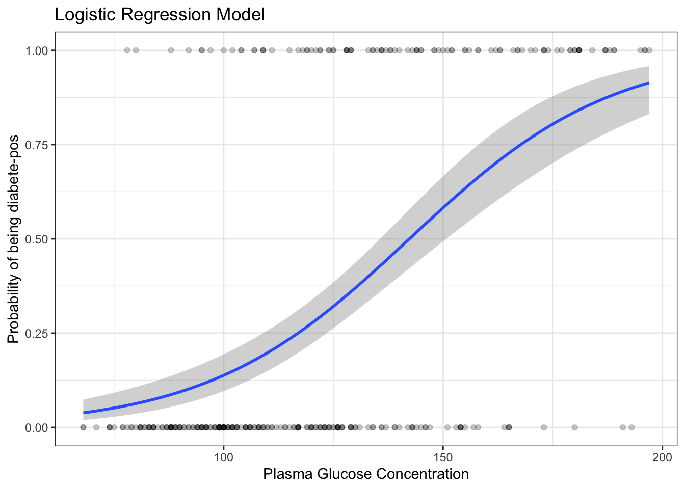
model <- glm( diabetes ~ glucose + mass + pregnant,
              data = train.data, family = binomial)
summary(model)$coef
Estimate Std. Error z value Pr(>|z|)
(Intercept) -9.32369818 1.125997285 -8.280391 1.227711e-16
glucose 0.03886154 0.005404219 7.190962 6.433636e-13
mass 0.09458458 0.023529905 4.019760 5.825738e-05
pregnant 0.14466661 0.045125729 3.205857 1.346611e-03 Estimate Std. Error z value Pr(>|z|)
(Intercept) -1.053400e+01 1.439679266 -7.31690975 2.537464e-13
pregnant 1.005031e-01 0.061266974 1.64041157 1.009196e-01
glucose 3.709621e-02 0.006486093 5.71934633 1.069346e-08
pressure -3.875933e-04 0.013826185 -0.02803328 9.776356e-01
triceps 1.417771e-02 0.019981885 0.70952823 4.779967e-01
insulin 5.939876e-04 0.001508231 0.39383055 6.937061e-01
mass 7.997447e-02 0.031798907 2.51500698 1.190300e-02
pedigree 1.329149e+00 0.482291020 2.75590704 5.852963e-03
age 2.718224e-02 0.020199295 1.34570257 1.783985e-01coef(model) (Intercept) pregnant glucose pressure triceps
-1.053400e+01 1.005031e-01 3.709621e-02 -3.875933e-04 1.417771e-02
insulin mass pedigree age
5.939876e-04 7.997447e-02 1.329149e+00 2.718224e-02 model <- glm( diabetes ~ pregnant + glucose + pressure + mass + pedigree,
data = train.data, family = binomial)
probabilities <- model %>% predict(test.data, type = "response")
head(probabilities) 19 21 32 55 64 71
0.1352603 0.5127526 0.6795376 0.7517408 0.2734867 0.1648174 contrasts(test.data$diabetes) pos
neg 0
pos 1 19 21 32 55 64 71
"neg" "pos" "pos" "pos" "neg" "neg" mean(predicted.classes == test.data$diabetes)[1] 0.7564103library("mgcv")Loading required package: nlme
Attaching package: 'nlme'
The following object is masked from 'package:dplyr':
collapse
This is mgcv 1.8-42. For overview type 'help("mgcv-package")'.# Fit the model
gam.model <- gam(diabetes ~ s(glucose) + mass + pregnant,
data = train.data, family = "binomial")
# Summarize model
summary(gam.model )
Family: binomial
Link function: logit

Formula:
diabetes ~ s(glucose) + mass + pregnant

Parametric coefficients:
            Estimate Std. Error z value Pr(>|z|)
(Intercept) -4.59794    0.86982  -5.286 1.25e-07 ***
mass         0.09458    0.02353   4.020 5.83e-05 ***
pregnant     0.14467    0.04513   3.206  0.00135 **
---
Signif. codes:  0 '***' 0.001 '**' 0.01 '*' 0.05 '.' 0.1 ' ' 1

Approximate significance of smooth terms:
           edf Ref.df Chi.sq p-value
s(glucose)   1      1  51.71  <2e-16 ***
---
Signif. codes:  0 '***' 0.001 '**' 0.01 '*' 0.05 '.' 0.1 ' ' 1

R-sq.(adj) =  0.339   Deviance explained = 29.8%
UBRE = -0.083171  Scale est. = 1         n = 314
# Make predictions
probabilities <- gam.model %>% predict(test.data, type = "response")
predicted.classes <- ifelse(probabilities> 0.5, "pos", "neg")
# Model Accuracy
mean(predicted.classes == test.data$diabetes)[1] 0.7820513optional ========================================================================
Example implementation from scratch:
library(ggplot2)
library(dplyr)


N <- 200 # number of points per class
D <- 2 # dimensionality, we use 2D data for easy visualization
K <- 2 # number of classes, binary for logistic regression
X <- data.frame() # data matrix (each row = single example, can view as xy coordinates)
y <- data.frame() # class labels

set.seed(56)

t <- seq(0,1,length.out = N)
for (j in (1:K)){
  # t, m are parameters of parametric equations x1, x2
  # t <- seq(0,1,length.out = N)
  # add randomness
  m <- rnorm(N, j+0.5, 0.25)
  Xtemp <- data.frame(x1 = 3*t , x2 = m - t)
  ytemp <- data.frame(matrix(j-1, N, 1))
  X <- rbind(X, Xtemp)
  y <- rbind(y, ytemp)
}

data <- cbind(X,y)
colnames(data) <- c(colnames(X), 'label')

# create dir images
#dir.create(file.path('.', 'images'), showWarnings = FALSE)

# lets visualize the data:
data_plot <- ggplot(data) + geom_point(aes(x=x1, y=x2, color = as.character(label)), size = 2) +
  scale_colour_discrete(name  ="Label") +
  ylim(0, 3) + coord_fixed(ratio = 1) +
  ggtitle('Data to be classified') +
  theme_bw(base_size = 12) +
  theme(legend.position=c(0.85, 0.87))

#png(file.path('images', 'data_plot.png'))
print(data_plot)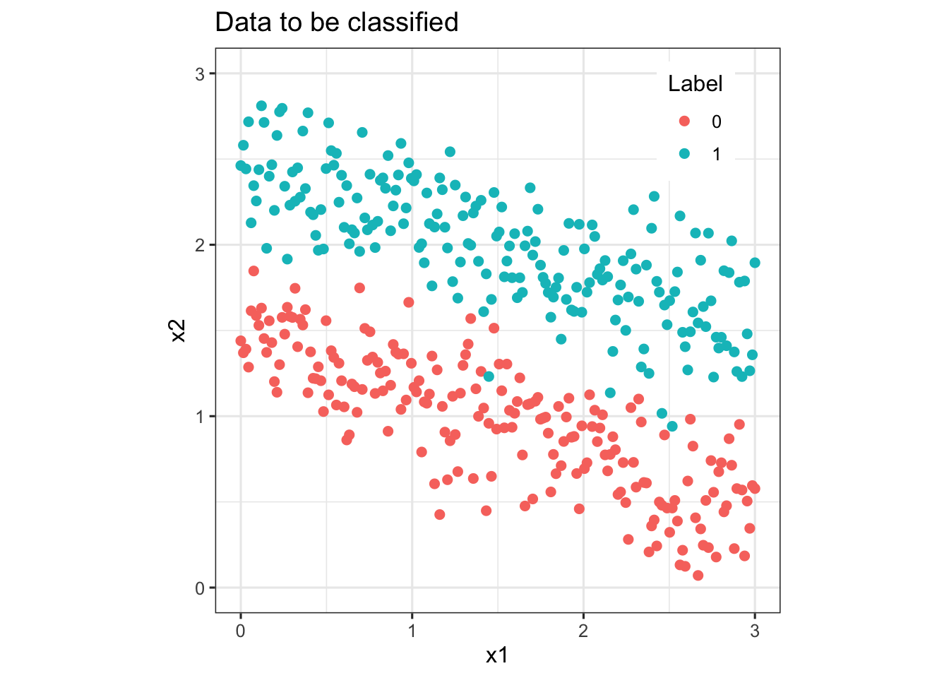
#dev.off()

#sigmoid function, inverse of logit
sigmoid <- function(z){1/(1+exp(-z))}

#cost function
cost <- function(theta, X, y){
  m <- length(y) # number of training examples
  h <- sigmoid(X %*% theta)
  J <- (t(-y)%*%log(h)-t(1-y)%*%log(1-h))/m
  J
}

#gradient function
grad <- function(theta, X, y){
  m <- length(y)

  h <- sigmoid(X%*%theta)
  grad <- (t(X)%*%(h - y))/m
  grad
}

logisticReg <- function(X, y){
  #remove NA rows
  X <- na.omit(X)
  y <- na.omit(y)
  #add bias term and convert to matrix
  X <- mutate(X, bias =1)
  #move the bias column to col1
  X <- as.matrix(X[, c(ncol(X), 1:(ncol(X)-1))])
  y <- as.matrix(y)
  #initialize theta
  theta <- matrix(rep(0, ncol(X)), nrow = ncol(X))
  #use the optim function to perform gradient descent
  costOpti <- optim(theta, fn = cost, gr = grad, X=X, y=y)
  #return coefficients
  return(costOpti$par)
}

logisticProb <- function(theta, X){
  X <- na.omit(X)
  #add bias term and convert to matrix
  X <- mutate(X, bias =1)
  X <- as.matrix(X[,c(ncol(X), 1:(ncol(X)-1))])
  return(sigmoid(X%*%theta))
}

logisticPred <- function(prob){
  return(round(prob, 0))
}

# training
theta <- logisticReg(X, y)
prob <- logisticProb(theta, X)
pred <- logisticPred(prob)

# generate a grid for decision boundary, this is the test set
grid <- expand.grid(seq(0, 3, length.out = 100), seq(0, 3, length.out = 100))
# predict the probability
probZ <- logisticProb(theta, grid)
# predict the label
Z <- logisticPred(probZ)
gridPred = cbind(grid, Z)

# decision boundary visualization
p <- ggplot() + geom_point(data = data, aes(x=x1, y=x2, color = as.character(label)), size = 2, show.legend = F) +
  geom_tile(data = gridPred, aes(x = grid[, 1],y = grid[, 2], fill=as.character(Z)), alpha = 0.3, show.legend = F)+
  ylim(0, 3) +
  ggtitle('Decision Boundary for Logistic Regression') +
  coord_fixed(ratio = 1) +
  theme_bw(base_size = 12)

#png(file.path('images', 'logistic_regression.png'))
print(p)
Warning: Removed 200 rows containing missing values (`geom_tile()`).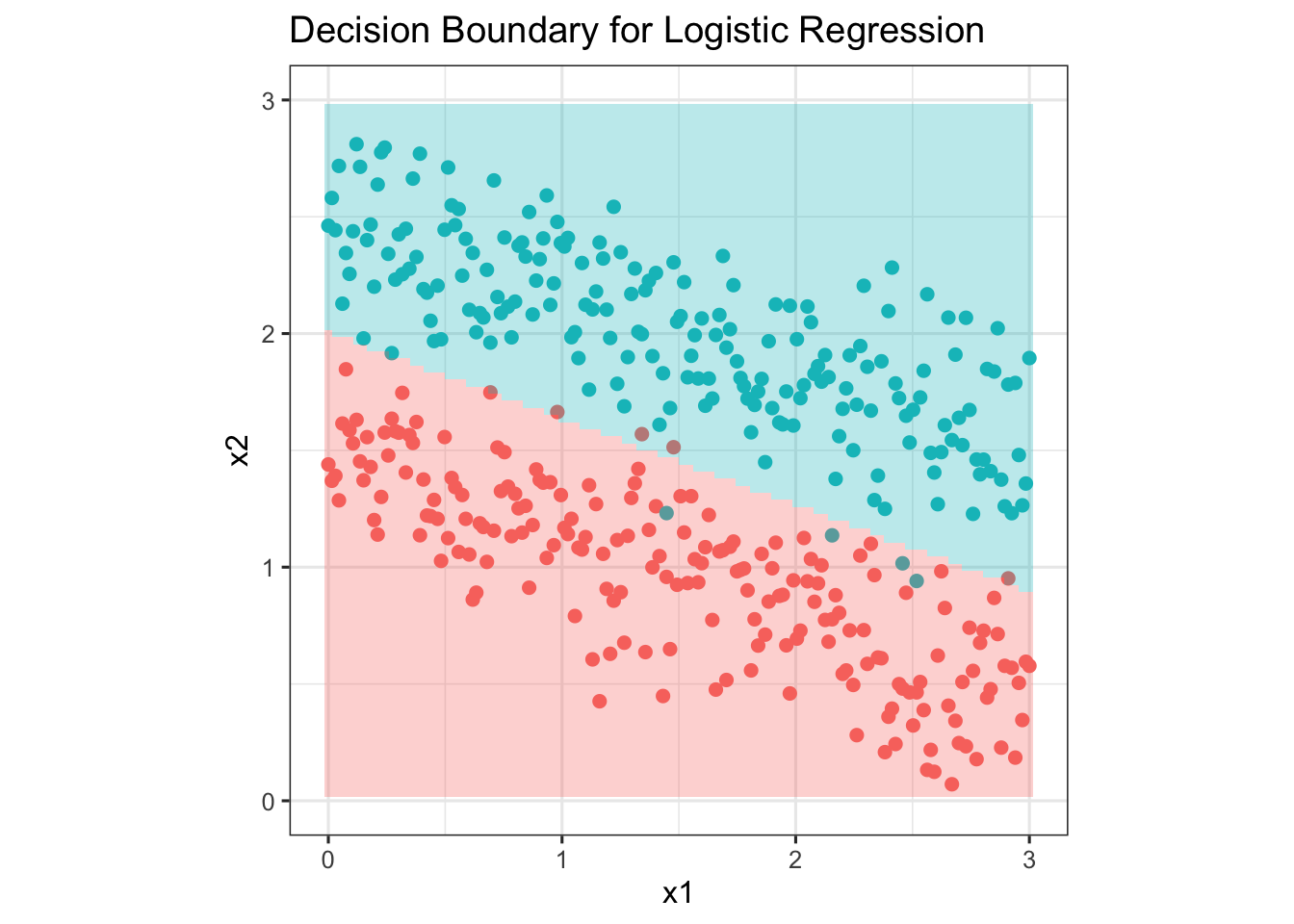
#dev.off()