Mean Sum of Squared Error
Lets implement this loss function in R and test it with our diabetes data.
Load diabetes dataset, lets make the dataset even smaller so we can properly understand
data("PimaIndiansDiabetes")

Data <- PimaIndiansDiabetes %>%
  select(age, glucose, mass) %>%
  add_rownames(var = "Patient ID")
Warning: `add_rownames()` was deprecated in dplyr 1.0.0.
ℹ Please use `tibble::rownames_to_column()` instead.DataSmaller <- Data[1:3,]
x <- DataSmaller$age
y <- DataSmaller$glucoseNow lets implement the function:
\[ \text{MSE} = \frac{1}{m} \sum_{i=1}^{m} \left( y_i - \left( \hat{\beta}_0 + \hat{\beta}_1 x_i \right) \right)^2 \]
mse_practical <- function(beta0, beta1, x, y, m) {
  (1 / m) * sum((y - (beta0 + beta1 * x))^2)
}
Put it to test with beta values B0 = 3 and B1 = 5 , then try with B0 = 4 and B1 = 7. Do it in a piece of paper by hand too. Remember, we already have the y, x and m values defined.
age <- DataSmaller$age
glucose <- DataSmaller$glucose
DataPoints <- length(x)

mse_practical(3, 5, age, glucose, DataPoints)
[1] 5584.667Remember this is the same as:
mse_practical(beta0 = 3, beta1 = 5, x = age, y= glucose, m =DataPoints)[1] 5584.667Now calculate it by hand!
 Repeat process with B0 = 4 and B1 = 7.
Click here to reveal the solution
mse_practical(beta0 = 4, beta1 = 7, x = age, y= glucose, m =DataPoints)[1] 20985.67Now lets understand how this translated to the linear regression model we are building
As you can see in this plot we have two lines with the slopes previously selected. The one with the lower loss fits the data better.
ggplot(DataSmaller, aes(x = age, y = glucose)) +
  geom_point() +
  geom_abline(slope = 3, intercept = 5, color = "blue", size = 1) +
  geom_abline(slope = 4, intercept = 7, color = "red", size = 1) +
  xlim(0, 80) +
  ylim(0, 300) +
  labs(title = "Different betas",
       x = "Age", y = "Glucose") +
  theme_minimal()
Warning: Using `size` aesthetic for lines was deprecated in ggplot2 3.4.0.
ℹ Please use `linewidth` instead.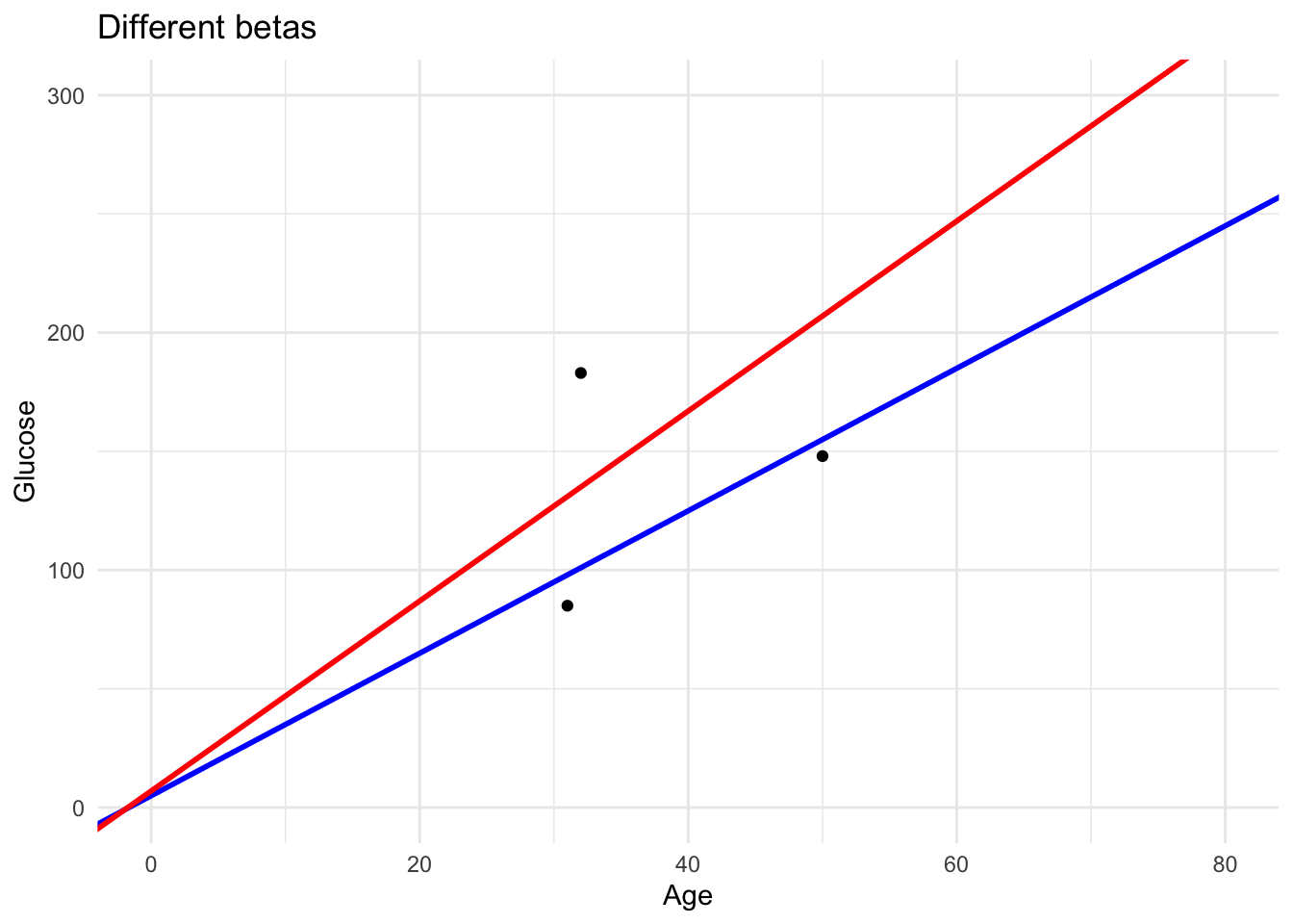
We could try this out for a range of different parameters. But, very slow.
For example lets go back to more data points:
DataSmaller <- Data[1:80,]

B0_values <- seq(10, 60, by = 20)
B1_values <- seq(0.5, 8, by = 2)

x_range <- seq(min(DataSmaller$age), max(DataSmaller$age), length.out = 100)


line_data <- expand.grid(B0 = B0_values, B1 = B1_values) %>%
  group_by(B0, B1) %>%
  do(data.frame(x = x_range, y = .$B0 + .$B1 * x_range)) %>%
  ungroup() %>%
  mutate(label = paste("B0 =", B0, ", B1 =", B1))
# Plot the original data points with the different regression lines

ggplot(DataSmaller, aes(x = age, y = glucose)) +
  geom_point(color = "black", size = 3) +  # Original data points
  geom_line(data = line_data, aes(x = x, y = y, color = label, linetype = label), size = 1) +
  labs(title = "Effect of Different B0 and B1 Values on the Regression Line",
       x = "Age (Predictor)", y = "Glucose (Response)",
       color = "Parameter Combination", linetype = "Parameter Combination") +
  theme_minimal()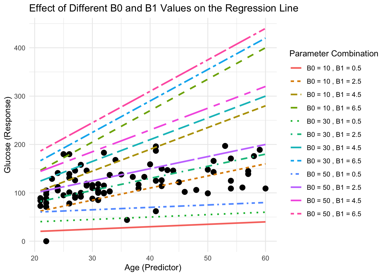
We need a way in which to find the combination of parameters that yields the minimum value of the loss function and so the linear regression model that best fits the data points. But what is the minimum of the loss function?
Lets plot the function for us to understand it better! As the function under study we need a 3D plot.
\[ MSE(\hat{\beta}_0, \hat{\beta}_1) = \frac{1}{m} \sum_{i=1}^{m} \left( y_i - \left( \hat{\beta}_0 + \hat{\beta}_1 x_i \right) \right)^2 \]
Using same betas as above
We can calculate the MSE for each combination (same way as we did by hand before) and store it in a matrix
names(B0_values) <- paste(B0_values,"(B0):", sep = "")
names(B1_values) <- paste(B1_values,"(B1):", sep = "")
mse_matrix <- outer(B0_values, B1_values, Vectorize(function(B0, B1) mse_practical(B0, B1, x =DataSmaller$age, y = DataSmaller$glucose, m=length(DataSmaller$glucose))))

head(mse_matrix)
0.5(B1): 2.5(B1): 4.5(B1): 6.5(B1):
10(B0): 9743.837 1694.788 4585.338 18415.49
30(B0): 6426.338 1197.288 6907.838 23557.99
50(B0): 3908.838 1499.788 10030.338 29500.49Try it for one of these combinations
mse_practical(beta0 = 10, beta1 = 0.5, x = age, y= glucose, m =DataPoints)[1] 13652.75Now lets plot this function!
par(mfrow = c(4, 1),  mgp = c(2.5, 0.8, 0))  # 2x2 layout

# 3D surface plot for SSE as a function of B0 and B1
persp3D(x = B0_values, y = B1_values, z = mse_matrix,
        xlab = "B0 (Intercept)", ylab = "B1 (Slope)", zlab = "MSE",
        main = "3D Surface Plot of MSE as a Function of B0 and B1",
        col = terrain.colors(50), theta = 40, phi = 20,
        ticktype = "detailed",    # Simplifies tick marks
        cex.axis = 0.8,         # Reduces axis label size
        cex.lab = 0.9,          # Reduces axis title size
        nticks = 5)

persp3D(x = B0_values, y = B1_values, z = mse_matrix,
        xlab = "B0 (Intercept)", ylab = "B1 (Slope)", zlab = "MSE",
        col = terrain.colors(50), theta = 290, phi = 20,
        ticktype = "detailed")

persp3D(x = B0_values, y = B1_values, z = mse_matrix,
        xlab = "B0 (Intercept)", ylab = "B1 (Slope)", zlab = "MSE",
        col = terrain.colors(50), theta = 60, phi = 10,
        ticktype = "detailed")


persp3D(x = B0_values, y = B1_values, z = mse_matrix,
        xlab = "B0 (Intercept)", ylab = "B1 (Slope)", zlab = "MSE",
        col = terrain.colors(50), theta = 90, phi = 200,
        ticktype = "detailed")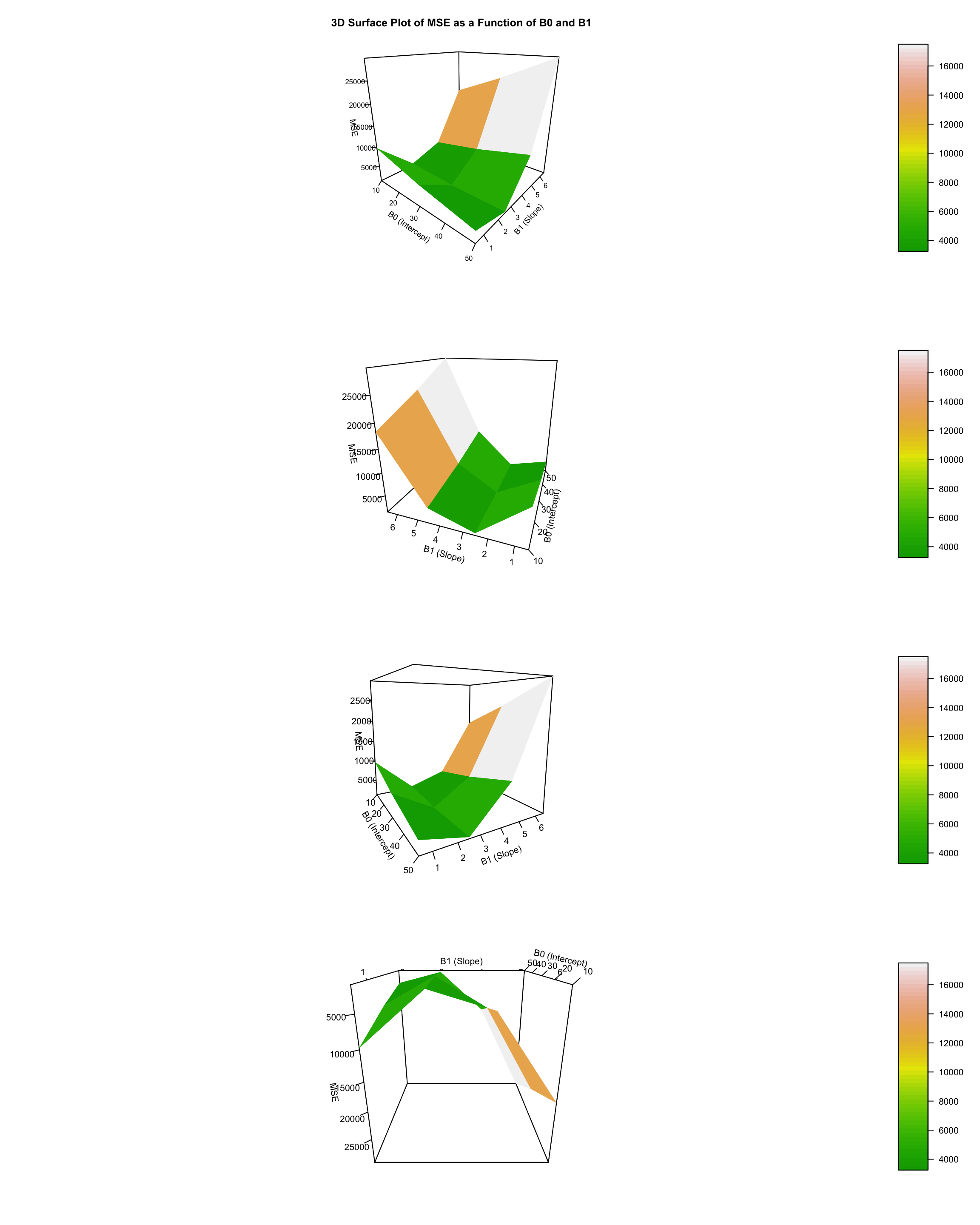
What is the minimum MSE? This one! Roughly we can see that it corresponds to around x. What we also find from here is the idea that the minim point is the one at the bottom of the 3D curved surface.
plot.new()

persp3D(x = B0_values, y = B1_values, z = mse_matrix,
        xlab = "B0 (Intercept)", ylab = "B1 (Slope)", zlab = "MSE",
        main = "3D Surface Plot of MSE as a Function of B0 and B1",
        col = terrain.colors(50), theta = 40, phi = 20,
        ticktype = "detailed",   # Simplifies tick marks
        cex.axis = 0.8,          # Reduces axis label size
        cex.lab = 0.9,           # Reduces axis title size
        nticks = 5)

# Find the minimum point in the mse_matrix
min_index <- which(mse_matrix == min(mse_matrix), arr.ind = TRUE)
min_B0 <- B0_values[min_index[1]]
min_B1 <- B1_values[min_index[2]]
min_mse <- min(mse_matrix)

# Add a point at the minimum location
points3D(x = min_B0, y = min_B1, z = min_mse,
         col = "red", pch = 19, cex = 1.5, add = TRUE)

# Add a label for the minimum point
text3D(x = min_B0+4, y = min_B1+ 15, z = min_mse + 0.5,
       labels = paste("Min MSE\n(B0 =", round(min_B0, 2),
                      ", B1 =", round(min_B1, 2), ")"),
       col = "red", add = TRUE)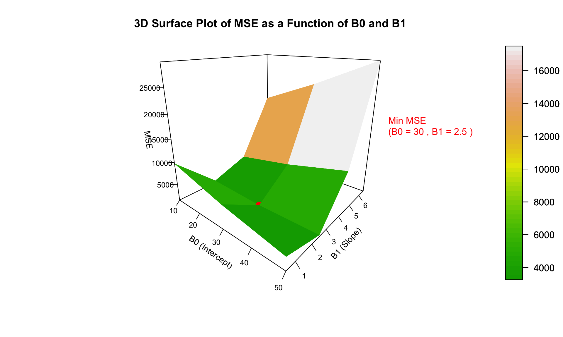
If we were to go back to fitting the line using lm as as the start we would get:
lm(glucose ~ age, data = DataSmaller)
Call:
lm(formula = glucose ~ age, data = DataSmaller)

Coefficients:
(Intercept)          age
      73.68         1.33
2D plots
Finally, visualization in 3D complex. Lets understand next stepsg oing back to 2D planes. For the MSE function we can go back to a 2D plane, by fixing one of the betas, imagine we know B0 is the one that offers this minimum (intercept/B0 = 70), so now lets try and explore what B1 makes it the minimum too.
# Set a fixed slope (B1) based on an estimated model
fixed_B0 <- lm(glucose ~ age, data = DataSmaller)$coefficients[1]

# Generate a range of B0 values and calculate SSE for each B0
B1_values <- seq(-3, 5, length.out = 100)
sse_values <- sapply(B1_values, function(B1) mse_practical(fixed_B0, B1, DataSmaller$age,DataSmaller$glucose, length(DataSmaller$glucose)))

# Plot SSE as a function of B0
ggplot(data.frame(B1 = B1_values, SSE = sse_values), aes(x = B1, y = SSE)) +
  geom_line(color = "blue") +
  geom_point(aes(x = B1_values[which.min(sse_values)], y = min(sse_values)), color = "red", size = 3) +
  labs(title = "2D Plot of SSE as a Function of B0 (Intercept)", x = "B1 (Slope)", y = "Mean Squared Error (MSE)") +
  theme_minimal()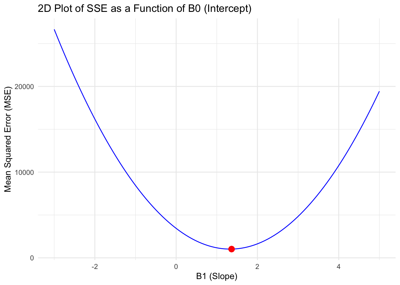
Quadratic function!
# Generate data for different intercepts (B0 values) with fixed slope (B1)
B1_samples <- c(min(B1_values), round(B1_values[which.min(sse_values)],3), max(B1_values))
line_data <- do.call(rbind, lapply(B1_samples, function(B1) data.frame(x = DataSmaller$age, y = fixed_B0 + B1 * DataSmaller$age, B1 = B1)))

# Plot the original data with different fitted lines
ggplot(DataSmaller, aes(x = age, y = glucose)) +
  geom_point(color = "black", size = 3) +
  geom_line(data = line_data, aes(x = x, y = y, color = factor(B1)), size = 1) +
  labs(title = "Effect of Changing B0 (Intercept) on Linear Regression Line", color = "B0 (Intercept)") +
  theme_minimal()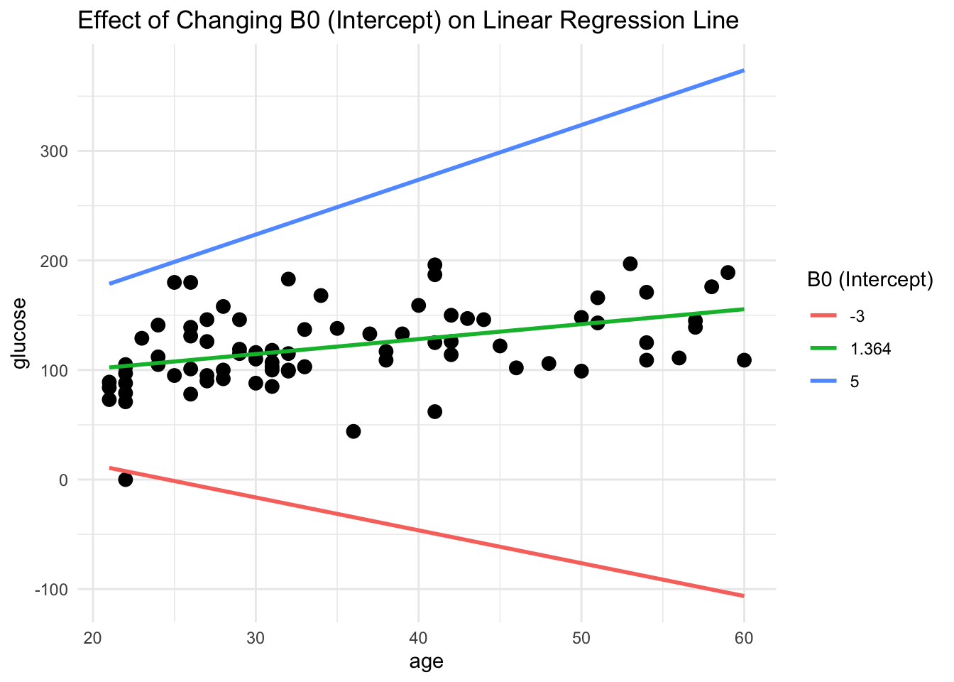
Which was exactly what calculated above!
lm(glucose ~ age, data = DataSmaller)
Call:
lm(formula = glucose ~ age, data = DataSmaller)

Coefficients:
(Intercept)          age
      73.68         1.33
Maps to what we saw in 3D surface, same Betas! (Have to do it with more data points!)
Key is, we have created an intutiton. To find minim of loss function, we need to fin a way n which to find the cnvex point. And we can do it through derivatives!!
Key is, we have created an intutiton. To find minim of loss function, we need to fin a way n which to find the cnvex point. And we can do it through derivatives!!
Remember to save your work frequently!
Back to slides
This is a custom div block. You can style it by defining a CSS class in the Quarto project.
Back to the slides
This text is large and blue.
Custom styled box: You can use HTML and CSS to customize text further.
Slope, derivatives of examples = 0, log, saddle point etc.
Derivative of loss function - calculate
Gradient descent.
DONE!