# Import necessary libraries
import pandas as pd
import numpy as np
from sklearn.linear_model import LogisticRegression
import matplotlib.pyplot as plt
from sklearn.datasets import fetch_openml(1b) Fitting a logistic regression model - Python
# Load the Pima Indians Diabetes dataset
data = fetch_openml(name="diabetes", version=1, as_frame=True)
/Users/bravol/Library/r-miniconda/envs/r-reticulate/lib/python3.8/site-packages/sklearn/datasets/_openml.py:1022: FutureWarning: The default value of `parser` will change from `'liac-arff'` to `'auto'` in 1.4. You can set `parser='auto'` to silence this warning. Therefore, an `ImportError` will be raised from 1.4 if the dataset is dense and pandas is not installed. Note that the pandas parser may return different data types. See the Notes Section in fetch_openml's API doc for details.
warn(PimaIndiansDiabetes = data.frameWe have some different names (plas is glucose in R), but same idea.
# Select relevant features and target variable
PimaIndiansDiabetes = PimaIndiansDiabetes[["plas", "class", "mass", "age"]]
# Define predictor (X) and target (y) variables
X = PimaIndiansDiabetes[["plas"]]
y = PimaIndiansDiabetes["class"]# Fit a logistic regression model using sklearn
logistic_model = LogisticRegression()
logistic_model.fit(X, y)LogisticRegression()In a Jupyter environment, please rerun this cell to show the HTML representation or trust the notebook.
On GitHub, the HTML representation is unable to render, please try loading this page with nbviewer.org.
LogisticRegression()
# Display model coefficients
intercept = logistic_model.intercept_[0]
slope = logistic_model.coef_[0][0]
print(f"Intercept: {intercept}, Slope: {slope}")
Intercept: -5.350028074882648, Slope: 0.037872619821980175# Predict probabilities
PimaIndiansDiabetes["predicted_probability"] = logistic_model.predict_proba(X)[:, 1]<string>:1: SettingWithCopyWarning:
A value is trying to be set on a copy of a slice from a DataFrame.
Try using .loc[row_indexer,col_indexer] = value instead
See the caveats in the documentation: https://pandas.pydata.org/pandas-docs/stable/user_guide/indexing.html#returning-a-view-versus-a-copyPimaIndiansDiabetes.head() plas class mass age predicted_probability
0 148.0 tested_positive 33.6 50.0 0.563436
1 85.0 tested_negative 26.6 31.0 0.106134
2 183.0 tested_positive 23.3 32.0 0.829298
3 89.0 tested_negative 28.1 21.0 0.121387
4 137.0 tested_positive 43.1 33.0 0.459718# Visualise predictions
plt.figure(figsize=(8, 6))
plt.scatter(PimaIndiansDiabetes["plas"], PimaIndiansDiabetes["class"], alpha=0.5, label="Actual")
plt.scatter(PimaIndiansDiabetes["plas"], PimaIndiansDiabetes["predicted_probability"], color="red", alpha=0.5, label="Predicted")
plt.plot(
np.sort(PimaIndiansDiabetes["plas"]),
np.sort(logistic_model.predict_proba(X)[:, 1]),
color="blue",
label="Logistic Regression Curve"
)
plt.xlabel("Glucose")
plt.ylabel("Diabetes (0 or 1)")
plt.title("Logistic Regression: Glucose vs Diabetes")
plt.legend()
plt.grid(alpha=0.3)
plt.show()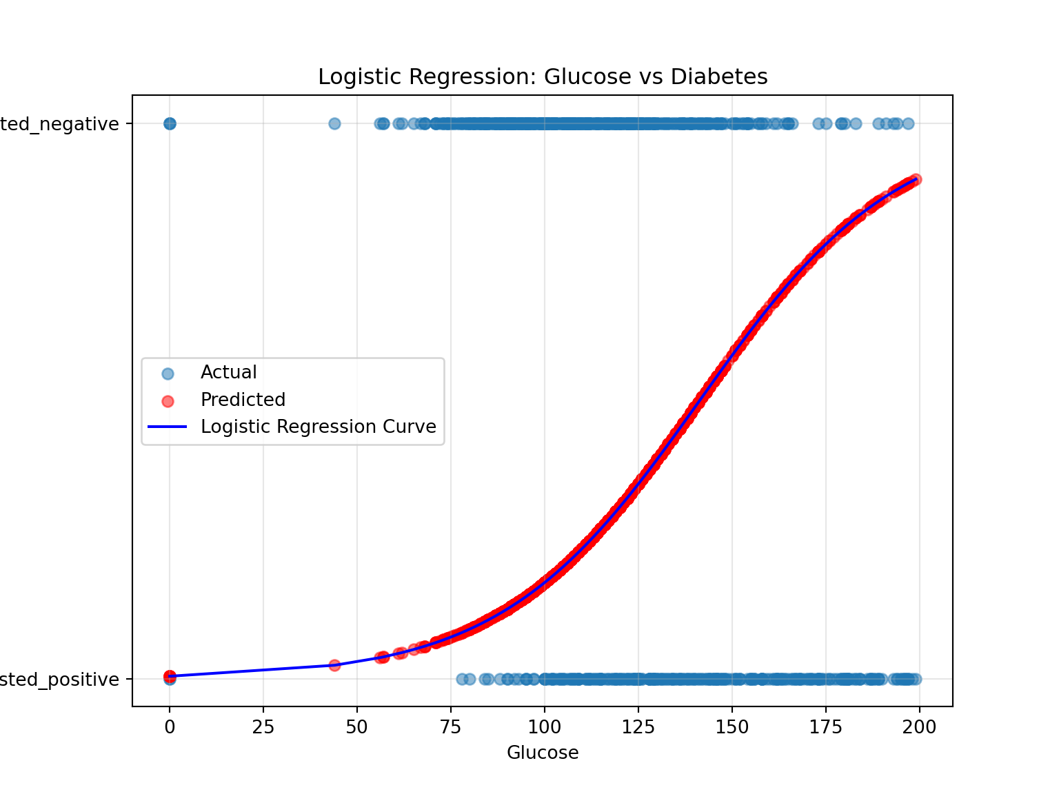
Now include more predictors: “plas” and “age”
# Fit logistic regression with multiple predictors
X_multi = PimaIndiansDiabetes[["plas", "age"]]
logistic_model_two = LogisticRegression()
logistic_model_two.fit(X_multi, y)LogisticRegression()In a Jupyter environment, please rerun this cell to show the HTML representation or trust the notebook.
On GitHub, the HTML representation is unable to render, please try loading this page with nbviewer.org.
LogisticRegression()
# Display model coefficients
intercept = logistic_model_two.intercept_[0]
slope = logistic_model_two.coef_[0][0]
print(f"Intercept: {intercept}, Slope: {slope}")
Intercept: -5.912369223097624, Slope: 0.03564371909912629# Predict probabilities for the multi-feature model
PimaIndiansDiabetes["predicted_probability_two"] = logistic_model_two.predict_proba(X_multi)[:, 1]<string>:1: SettingWithCopyWarning:
A value is trying to be set on a copy of a slice from a DataFrame.
Try using .loc[row_indexer,col_indexer] = value instead
See the caveats in the documentation: https://pandas.pydata.org/pandas-docs/stable/user_guide/indexing.html#returning-a-view-versus-a-copyVisualize the probabilities
PimaIndiansDiabetes.head() plas class ... predicted_probability predicted_probability_two
0 148.0 tested_positive ... 0.563436 0.646059
1 85.0 tested_negative ... 0.106134 0.107690
2 183.0 tested_positive ... 0.829298 0.802707
3 89.0 tested_negative ... 0.121387 0.097990
4 137.0 tested_positive ... 0.459718 0.447313
[5 rows x 6 columns]Add mass to the modeling too (so in total three predictors, one outcome variable), how do the predictions change?
Back to top