Probability: 0.8Odds: 4.0Log-Odds: 1.4First lets start with setting probabilities, odds and log odds and seeing how they are all related:
Probability: 0.8Odds: 4.0Log-Odds: 1.4Now, lets fit a logistic regression model. As we said yesterday, the learning algorithm is already coded for us! So we just have to apply the correct function. In this case we will use glm() and set as input parameters family = binomial https://www.rdocumentation.org/packages/stats/versions/3.6.2/topics/glm, https://www.rdocumentation.org/packages/stats/versions/3.6.2/topics/family which specifies implementing a logistic regression algorithm by setting the link function to logit . We could have also used any of the models in tidymodels https://parsnip.tidymodels.org/reference/logistic_reg.html
The data we will be using is the same as yesterday’s, PimaIndiansDiabetes
Attaching package: 'dplyr'The following objects are masked from 'package:stats':
filter, lagThe following objects are masked from 'package:base':
intersect, setdiff, setequal, union pregnant glucose pressure triceps insulin mass pedigree age diabetes
1 6 148 72 35 0 33.6 0.627 50 pos
2 1 85 66 29 0 26.6 0.351 31 neg
3 8 183 64 0 0 23.3 0.672 32 pos
4 1 89 66 23 94 28.1 0.167 21 neg
5 0 137 40 35 168 43.1 2.288 33 pos
6 5 116 74 0 0 25.6 0.201 30 negWe have lots of features/columns, so lets narrow it down to just a few
neg and pos
table(PimaIndiansDiabetes$diabetes)
neg pos
500 268
For our first logistic regression model, we are going to just use glucose as predictor only. We can specify this in the following way:
# Fit a logistic regression model
logistic_model <- glm(diabetes ~ glucose, data = PimaIndiansDiabetes, family = binomial)

# View model summary
summary(logistic_model)
Call:
glm(formula = diabetes ~ glucose, family = binomial, data = PimaIndiansDiabetes)

Deviance Residuals:
    Min       1Q   Median       3Q      Max
-2.1096  -0.7837  -0.5365   0.8566   3.2726

Coefficients:
             Estimate Std. Error z value Pr(>|z|)
(Intercept) -5.350080   0.420827  -12.71   <2e-16 ***
glucose      0.037873   0.003252   11.65   <2e-16 ***
---
Signif. codes:  0 '***' 0.001 '**' 0.01 '*' 0.05 '.' 0.1 ' ' 1

(Dispersion parameter for binomial family taken to be 1)

    Null deviance: 993.48  on 767  degrees of freedom
Residual deviance: 808.72  on 766  degrees of freedom
AIC: 812.72

Number of Fisher Scoring iterations: 4
What is the predictive model we have fitted?
This one!
\[
P = \frac{1}{1 + \exp\left(-\left(-5.35 + 0.0379 \cdot \text{glucose}\right)\right)}
\] Where glm() has done all teh work for us, and identified the parameters \(B_0\) and \(B_1\) that best fit our dataset.These parameters are:
(Intercept)
   -5.35008
slope glucose
0.03787304 With this information, we could calcluate for example, the odds of having diabetes, if \(glucose = 120\)
#odds transformation
odds <- exp(intercept + slope * 120) # Example: glucose = 120
cat("Odds at glucose = 120:", odds, "\n")
Odds at glucose = 120: 0.4469466 Just as a side not, we want pos to be our predicted outcome, shpuld we ‘dummify’ the column so we have 0s and 1s only? Lets try and see:
PimaIndiansDiabetes$diabetes_dummy <- ifelse(PimaIndiansDiabetes$diabetes ==  "pos", 1, 0)
head(PimaIndiansDiabetes$diabetes_dummy)
[1] 1 0 1 0 1 0# Fit a logistic regression model
logistic_model <- glm(diabetes_dummy ~ glucose, data = PimaIndiansDiabetes, family = binomial)
# View model summary
summary(logistic_model)
Call:
glm(formula = diabetes_dummy ~ glucose, family = binomial, data = PimaIndiansDiabetes)

Deviance Residuals:
    Min       1Q   Median       3Q      Max
-2.1096  -0.7837  -0.5365   0.8566   3.2726

Coefficients:
             Estimate Std. Error z value Pr(>|z|)
(Intercept) -5.350080   0.420827  -12.71   <2e-16 ***
glucose      0.037873   0.003252   11.65   <2e-16 ***
---
Signif. codes:  0 '***' 0.001 '**' 0.01 '*' 0.05 '.' 0.1 ' ' 1

(Dispersion parameter for binomial family taken to be 1)

    Null deviance: 993.48  on 767  degrees of freedom
Residual deviance: 808.72  on 766  degrees of freedom
AIC: 812.72

Number of Fisher Scoring iterations: 4
We get the same results! glm recognizes this as a category and does it for us!
Now, lets make predictions. We are going to use our same dataset we used to fit our data, and see how much the predicted probabilities differ from the real/true classes. Again, we use the function predict.
predictions <- predict(logistic_model, type = "response")Lets add them to the dataset using tidyverse
# Add predictions to the dataset
PimaIndiansDiabetesWithPred <- PimaIndiansDiabetes %>%
  mutate(predicted_probability = predictions)

# Preview data with predictions
head(PimaIndiansDiabetesWithPred)
glucose diabetes mass age diabetes_dummy predicted_probability
1 148 pos 33.6 50 1 0.5634385
2 85 neg 26.6 31 0 0.1061322
3 183 pos 23.3 32 1 0.8293015
4 89 neg 28.1 21 0 0.1213849
5 137 pos 43.1 33 1 0.4597189
6 116 neg 25.6 30 0 0.2775177We do see a pattern right? Those with diabetes = pos (our 1) have higher probabilities. Lets double
# Step 4: Visualize results
library(ggplot2)

# Plot glucose vs. predicted probability
ggplot(PimaIndiansDiabetesWithPred, aes(x = glucose, y = diabetes_dummy)) +
  geom_point(alpha = 0.5) +
  geom_point(aes(x = glucose, y = predicted_probability),alpha = 0.5, colour = "red") +
  geom_smooth(method = "glm", method.args = list(family = binomial), se = FALSE) +
  labs(
       x = "Glucose",
       y = "Diabetes") +
  theme_minimal()
`geom_smooth()` using formula = 'y ~ x'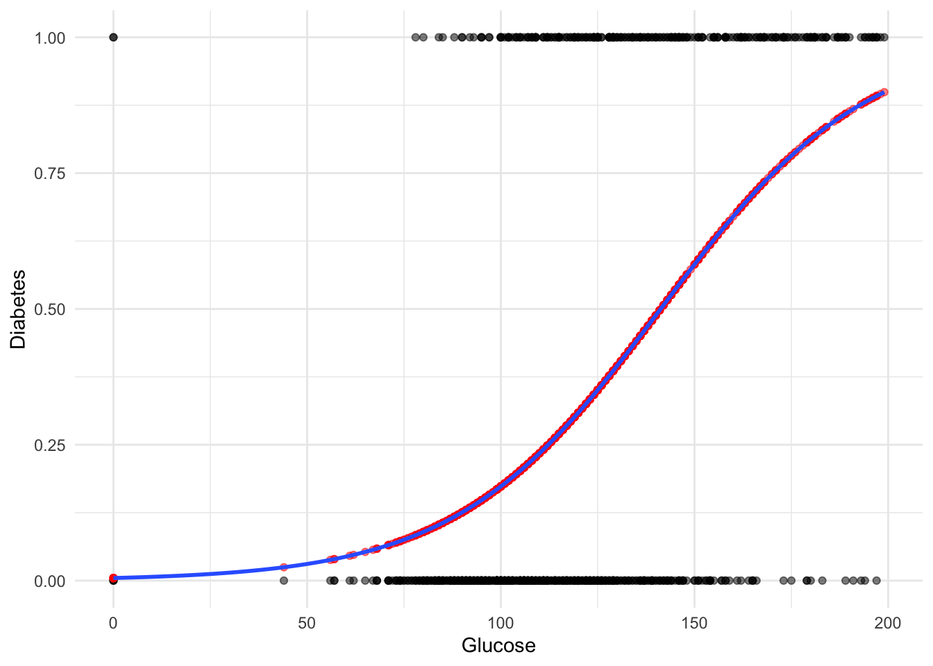
Now build a logistic regression model with more features. Include glucose + age + mass. Compare predictions!
# Fit a logistic regression model
logistic_model_three <- glm(diabetes_dummy ~ glucose + age + mass, data = PimaIndiansDiabetes, family = binomial)

# View model summary
summary(logistic_model_three)
Call:
glm(formula = diabetes_dummy ~ glucose + age + mass, family = binomial,
    data = PimaIndiansDiabetes)

Deviance Residuals:
    Min       1Q   Median       3Q      Max
-2.3809  -0.7476  -0.4357   0.7861   2.8263

Coefficients:
             Estimate Std. Error z value Pr(>|z|)
(Intercept) -8.393743   0.666067 -12.602  < 2e-16 ***
glucose      0.032512   0.003329   9.767  < 2e-16 ***
age          0.030157   0.007632   3.951 7.77e-05 ***
mass         0.081590   0.013526   6.032 1.62e-09 ***
---
Signif. codes:  0 '***' 0.001 '**' 0.01 '*' 0.05 '.' 0.1 ' ' 1

(Dispersion parameter for binomial family taken to be 1)

    Null deviance: 993.48  on 767  degrees of freedom
Residual deviance: 755.68  on 764  degrees of freedom
AIC: 763.68

Number of Fisher Scoring iterations: 5#Continue!Now lets do the same in python.
Back to top